WIXLIB

HAN AND WESTWATER: ANALYSIS AND IMPROVEMENT OF TIPPING CALIBRATIONNOAA’s Environmental Technology Laboratory (ETL) operated two microwave radiometers at the CART site. Duringthe same time, NOAA’s forecast systems laboratory (FSL)operated two GPS’s, one at the SGP CF and one at NOAA’swind profiler site near Lamont, OK, about 9 km away fromthe CF. NASA’s Goddard Space Flight Center (NASA/GDFC),Greenbelt, MD, operated a Raman water vapor lidar, and theARM operational Raman lidar was operated as well. At the CF,ARM has also routinely operated an MWR for several years[7]. The primary goal of these deployments was to quantify theabsolute accuracies of the MWR’s and GPS’s in PWV and tocompare these measurements with in situ measurements madeevery 3 h by ARM’s balloon borne sounding systems (BBSS).Preliminary intercomparisons among these instruments showedthat the PWV from the ARM’s MWR was consistently higherthan that from all other instruments. With other instrumentsbeing in agreement with one another, a logical step was toexamine the calibration process performed on both ARM andETL MWR’s during the experiment. This led to the investigation of the calibration method that we present here.Microwave radiometers that are used in space are usually calibrated using known calibration reference targets [13]. However,it is desirable to have a target temperature close to the brightnesstemperatures that an MWR measures during regular observations. For the upward-looking radiometer channels consideredhere, the observed brightness temperature can be as low as 10K. Two calibration methods are often applied for these channels:using a liquid nitrogen LN -cooled blackbody target or a tippingcalibration method that uses a clear atmosphere as a calibrationreference. If applied with care and caution, the LN method canbe useful. However, it is not practical to be applied and automated in long-term, routine operations. With the tipping method[14], [15], the radiometer takes measurements at two or more elevation angles in a horizontally-stratified atmosphere. The calibration is accomplished by adjusting a single numerical calibration parameter that is required by the system software untilthe outputs of the system comply with a known physical relationship. In addition, as discussed in Section IV-G, strict qualitycontrol methods must also be applied to the data before the calibration parameter is changed. With suitable scanning, the calibration procedure can be automated. The ETL’s and ARM’sradiometer systems were all calibrated using the tipping calibration method during the experiment.The tipping method couples a radiometer equation that is specific to the radiometer in use and the theory of the radiativetransfer in the atmosphere. Calibration uncertainties may arisefrom both the system and the application of the theory. To investigate and reduce the uncertainties, we first take a simulationapproach to reveal problems and develop techniques to solvethem. We then apply these techniques to the data taken duringWVIOP’97. The simulations are based on radiosonde data collected around the area of the CART site. Although the data aresite specific, results of the analysis are general, and the techniques developed can be applied to all tipping calibrations.II. RADIATIVE TRANSFER AND RADIOMETER EQUATIONSThe fundamental quantity a radiometer measures is radiationpower, which is related to the specific intensity (or radiance) ,1261defined as the radiation power per unit area, per unit frequencyinterval at a specified frequency , and per unit solid angle ata specified direction. However, in the microwave frequency region, the intensity is usually expressed as brightness tempera. In microwave radiometry, there are twoture, denoted aspopular definitions of the brightness temperature. Because ofthe differences between these two difinitions, some confusionand mistakes may arise when measurements or models are compared. Because it is important to be aware of the issue, we include a brief discussion in the following. A detailed discussionis given in Janssen [16] and Stogryn [17].The so-called Rayleigh–Jeans equivalent brightness temperature is defined as(1)where , , and are the speed of light, Boltzmann’s constant,and frequency, respectively. Note that (1) is not the traditionalis a scaled intensity inRayleigh–Jeans approximation.temperature units. The second definition is the so-called thermodynamic brightness temperature, defined as(2)is the inverse of the Planck functionat awhere. The Planck functionis the radiancetemperatureemitted at from a blackbody at temperature and is given by(3)is an equivalent temperature atBy way of analogy,which a blackbody emits the amount of radiation at the intensity. The conversion fromtois(4),Unlikethe Planck functionis not linearly related to . Expandingin terms of, one obtains(5)where is the Planck constant. The first term is the traditionalRayleigh–Jeans approximation, and the second may be considered at a first-order correction to the Rayleigh–Jeans approxi, but only on frequency. Inmation and depends not onGHz, the first two terms are usually suffithe region, is very low (e.g.,cient for applications, except whenfor the cosmic background at 2.75 K). Thus, under normal conditions, for the amount of radiation received by ground-basedandis wellradiometers, the difference between, which is proporrepresented by the second term in (5),tional to frequency. At 20.6 GHz, this term has a value of 0.49 Kis as lowand 31.4 GHz, a value of 0.75 K. Even whenas the cosmic background at 2.75 K, the sum of the remainingterms is not significant for the frequencies considered here. ForK, the third term is equal to 0.030example, forK at 20.6 GHz and 0.069 K at 31.4 GHz. However, it may besignificant at higher frequencies.Authorized licensed use limited to: Susanne Crewell. Downloaded on March 29, 2009 at 09:05 from IEEE Xplore. Restrictions apply.

1262IEEE TRANSACTIONS ON GEOSCIENCE AND REMOTE SENSING, VOL. 38, NO. 3, MAY 2000Following Janssen [16], the definition ofmay be applied to scale the uplooking radiative transfer equation(6)whereis the optical path, andis the opacityat an elevation angle . The opacity is then calculated as [forconvenience, we will drop the symbol and express the opacity]asinto an equation with temperature units as(12)(7)is the cosmic background temperature and is awhereis defined asfunction of fequency, and(8)is not equal to the physical air temperature .Note thatThe radiometer equation relates the system output voltage toinput radiation power. Usually, an MWR system views one ormore internal or external blackbody targets for initial calibrations. Taking a simple example, if a linear system has two calibration reference targets at temperatures and , the intensity(averaged over an antenna beam) measured by the radiometerobserving the sky, may be given by the following radiometerequationNote that in (12), the sky brightness temperature is defined asusing (4) becausethat of the Rayleigh–Jeans equivalentit is defined as a thermodynamic brightness temperature. If weexpress each of the quantities in (12) in terms of the temperatures given by (4) and expand the Planck functions, we maycalculate the opacity as(13)after neglecting the third and higher terms, where(9)are detected voltages from the sources ofwhere , , andthe sky, target 1, and target 2, respectively. The radiometer equation may be scaled in the same way as that for obtaining the radiative transfer (7). Thus, the measurements given by the scaledradiometer equation are consistent with the radiative transferequation (7). Note that in the scaled equation, the quantities(or ) are not equal toor .It is common, however, that physical temperatures are directly used in the radiometer equations. This is done by linin terms of (i.e., using the first two terms inearizingthe expansion similar to (5)). If we substitute each of the radia,, andtion intensities,, whereandinto(9), we have(10)We see that this radiometer equation is consistent with themodel that computes the thermodynamic brightness temperabut is not consistent with the radiative transferture. As discussed earlier, under normal(7) that calculatesconditions, (10) is sufficient for applications. However, insituations such as zenith radiometric observations from aircraft, the atmospheric radiation power may be too low to belinearized in terms of the thermodynamic temperature and thus,the radiometer (10) may not be valid.In many applications of ground-based radiometry, includingtipping calibrations, there is a need to map the atmospheric radiation power into optical depth or opacity. This can be achievedafter defining a mean radiating temperature based on the radiative transfer equation (7)(11)(14)may be substituted with the measurementsIn (13),given by (10) directly. However, since (13) is an approximationof the exact (12), we should caution on the treatment of thequantity representing the cosmic background or sky brightness temperature with very low value. In some applications,neglecting the third term may not be valid.When mapping the measurements to opacity, it is importantthat the parameters in the mapping function be consistent withthe radiometer equation. For example, if the cosmic backgroundis given in Rayleigh–Jeans equivalent brightness temperature,and the sky temperature is given in thermodynamic brightnesstemperature, an inconsistency occurs that will fold a bias of 0.75K at 31.4 GHz into the calculation of opacity.The tipping calibration method is usually applied to determine the values of some constants in the radiometer equationthat models an MWR system’s input–output relationship. Weassume the MWR systems are linear and characterized by twoconstants such as a system gain and an offset [18]. If accuratecalibration reference targets are available at two temperaturesthat span the range of observable brightness temperatures, thenthe two constants can be determined. In many cases, the systemshave partial calibration information, with one of the constantsapproximately known, and leave the other to be determined inthe calibration processes. For example, the ETL radiometershave two internal calibration references, but the transmissionby a window and a segment of a waveguide need to be determined. In the following (and thereafter), we use the ETL’s andARM’s systems as examples to illustrate the tipping calibrationanalysis. The results are general for other types of radiometers.Each of the two ETL systems contains two independent microwave radiometers: one operates at 20.6 or 23.87 GHz and theother at 31.65 GHz. Other system parameters are listed in TableAuthorized licensed use limited to: Susanne Crewell. Downloaded on March 29, 2009 at 09:05 from IEEE Xplore. Restrictions apply.

HAN AND WESTWATER: ANALYSIS AND IMPROVEMENT OF TIPPING CALIBRATION1263TABLE ISELECTED RADIOMETER PARAMETERS: FREQUENCY (GHz), BANDWIDTH (GHz), –FULL WIDTHANTENNA PATTERN (DEGREES)I. Each radiometer has two internal blackbody loads, one at temperature , near 300 K, and the other at , about 100 K higherthan . The radiometer equation of the system is given as [14](15)is the antenna temperature [16], [17] being meawhereis the temperature of the radiometer waveguide, andsured,,, andare voltages of a square law detector, corresponding to the radiation sources of the two internal loads andthe sky, respectively. All these voltages and temperatures on theright side of the equation are measured. The unknown parameter is the parameter determined through the calibration and,as discussed in [14] and [18], describes transmission lossesdue to a portion of waveguide and a microwave window in thesystem.The ARM’s system operates at 23.8 and 31.4 GHz. Othermain system parameters are also listed in Table I. The system includes a noise diode injection device and an external blackbodyreference target at an ambient temperature . The radiometerequation of the system is given as [7](16)where is the voltage when the radiometer views the sky,is the voltage when viewing the reference target with the noiseis the voltage when viewing the reference with thediode on,is the noise injection temperature deternoise diode off, andmined through the calibration. The radiation loss and emissionof a microwave window in front of the radiometer antenna weremeasured in the laboratory and are assumed to be known and,, are simply incorpobecause they are multiplicative withrated into it.The radiometer (15) and (16) may be simplified for the sakeof convenience to simulate the tipping data. We may write theandin (16) as, whereparameters in (15) asandare correct calibration factors, and represents the, withreprecorrectness of the estimations of orsenting a perfect calibration. With this consideration, (15) or(16) may be rewritten in the form as(17)is an estimate of the true antenna temperaturewherein the pointing direction,for the ETL’s systems, andfor ARM’s system. We see that the measured antennawhen a caltemperature is equal to true antenna temperature). We will refer to theibration is performed without error (factor in (17) as the calibration factor. Equation (17) providesa convenient way to simulate the radiometric measurements inATHALF-MAXIMUM POWEROF THEwhich the atmospheric antenna temperaturemay be calculated using a radiative transfer and an antenna model. We will investigate the four frequency channels at 20.6, 22.235, 23.8, and31.4 GHz, respectively. Although the frequency channel 22.235GHz is not used in the ETL and ARM’s systems, it is includedhere for reference.III. TIPPING CALIBRATION METHODWe first define the atmospheric airmass as the ratio of the)opacity at the direction and the opacity at the zenith ((18)In (18), for convenience, we have dropped the frequency dependence in notation. The tipping calibration method uses measurements of opacity, derived from measurements of , as a function of airmass to derive a calibration factor. We will discussis derived from measurements of. Equationlater how(18) can be used to derive the calibration factor if the relationship between airmass and the observation angle is known.In a plane-stratified atmosphere and if we ignore the bendingof radiation rays caused by the gradient of refractive index, wehave(19)Sometimes, (19) is taken as the defining equation for airmass,but (18) is more general and includes (19) as a limiting case.Since (18) involves two opacities, the calibration procedure reand .quires observations of at least two different anglesandat the two anglesThe measurements,are then mapped into and in opacity space by using (12)or (13). Note that we have explicitly expressed the measurements as a function of the calibration factor . If we normalizeand by their corresponding airmasses asand, the normalized opacities and should theoretically have the same value, and any difference between them isdue to an incorrect calibration factor. We may adjust until anagreement between and is reached.The calibration factor may also be derived equally well inthe brightness temperature space. We may map the normalizedopacities and back to zenith brightness temperatures, reand.ferred to as normalized brightness temperatureThey too should be equal to one another. Any difference between them can be adjusted with the calibration factor . Theconcept of the normalized brightness temperature will be usedin later analysis.Authorized licensed use limited to: Susanne Crewell. Downloaded on March 29, 2009 at 09:05 from IEEE Xplore. Restrictions apply.

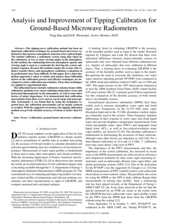
1264IEEE TRANSACTIONS ON GEOSCIENCE AND REMOTE SENSING, VOL. 38, NO. 3, MAY 2000To reduce measurement uncertainties, tipping observationsare often taken at more than two angles. Letbe the set of normalized opacities obtained from a set of observations. We may apply the least-square technique to obtain byminimizing the sum of square differences between any pair ofand,(;)opacities(20)where(21)Minimization with respect toyields the equation(22)whereFig. 1.Function given by (22), whose zero is the calibration factor.and(23)Solving (22), we obtain the calibration factor . Finding the zerois a well-posed mathematic problem as the curve ofof, shown in Fig. 1, suggests.We can look at the calibration procedure in anotherway. Tipping data is a set of airmass-opacity pairs. The basic idea is that if we, thenconsider as a function of ,(i.e., extrapolated to airmass 0 is 0). Thus, these points ofthe pairs lie on a straight line that must pass the origin on theairmass-opacity plane, and the slope of the line is the zenithopacity. If the fitted line does not pass the origin, it impliesan incorrect calibration factor. We may adjust the calibrationfactor until the line passes the origin. The mathematicalderivation is similar to the previous one. The difference is thatthe previous derivation minimizes the differences among thenormalized opacities, while the line fitting method minimizesthe differences between the opacities and a linear line thatpasses the origin. If only two angles are involved, the twomethods are identical.As pointed out by an anonymous reviewer, the metric of (20)could be replaced by a similar one involving the root-meansquare (rms) of the antenna temperature residuals. This metricwould result in giving an rms residual that could be comparedwith the noise level of the radiometer. However, the presentmethod could also give a similar rms residual after a mappingback from opacity space to antenna temperature space. Since thesame basic information enters into both metrics, we don’t thinkthat the results would differ substantially.There has been a less rigorous method that appears similar tothe second method. Since it has been often used [15], [19]–[21],it is worth a brief discussion here. The method fits a line to a setof tipping data with an approximate calibration factor . If theline’s offset is not equal to zero, the line’s slope is used as an approximation to the zenith opacity, which is then mapped into thezenith brightness temperature. Next, the zenith brightness temperature is used to obtain a new value of from the radiometerequation. The process may be repeated until the offset of the lineis near zero. The flaw of the method is that some of the information contained in the tipping data is lost in the process. Forexample, if the tipping observations are taken at angles with airmass 1, 2, and 3, the data at airmass 2 will never be used in thecalibration process.IV. CALIBRATION ERRORS AND METHODS TO REDUCE THEMCalibration errors may be caused by sources from the radiometer system and the violations of the assumptions in thetheory on which the calibration is based. The former include theeffect of radiometer antenna pattern, radiometer pointing errorand system random noise. The latter include the uncertainty inthe mean radiating temperature and the uncertainties in the fundamental relationship (19) between the airmass and the observation angles, which can be affected by nonstratified atmosphericconditions and the earth’s curvature.We simulated these error sources and developed and testedeffective techniques to reduce them. The simulations were performed by using a radiative transfer model [22] and the simplified radiometer (17) for a clear-sky atmosphere, which is represented by radiosonde pressure, temperature, and humidity profiles. A statistical ensemble of radiosonde data, referred to aswith a size of 16 380 soundings, was collected from five stationsaround the area of Oklahoma City, OK, from 1966 to 1992.To evaluate a calibration, we first need to define the calibra(the differencetion error. Although the quantity),between the calibration factor and its correct valuecan be used as a measure to the error, it may be more intuitive toexpress the error in terms of the brightness temperature. How-Authorized licensed use limited to: Susanne Crewell. Downloaded on March 29, 2009 at 09:05 from IEEE Xplore. Restrictions apply.

HAN AND WESTWATER: ANALYSIS AND IMPROVEMENT OF TIPPING CALIBRATION1265TABLE IICOLUMNS A: rms DIFFERENCES BETWEEN TWO MODEL CALCULATIONS OF T , ONE WITH REFRACTIVE INDEX CONSIDERED AND THE OTHER WITHOUT;COLUMNS B: rms DIFFERENCES BETWEEN TWO MODEL CALCULATIONS, ONE WITH EARTH CURVATURE CONSIDERED AND THE OTHER WITHOUT. THEDIFFERENCES (K) ARE LISTED AS A FUNCTION OF FREQUENCY (GHz) (ROW 1) AND AIRMASS (COLUMN 1)ever, for a given error, the error in corresponding antennatemperature depends on the magnitude of the temperature itself.For simplicity, we evaluate the error at a reference temperature. That is, for a calibration with an error, the calibrationerror is defined using (17) as(24)We use the climatological mean of the brightness temperatureas the reference temperature. The values of the reference temperatures are 27.2, 40.0, 35.0, and 18.5 K for the four selectedchannels at 20.6, 22.235, 23.8, and 31.4 GHz, respectively.Theoretically, any set of angles with two or more being distinct can be included in the tipping observations. However, because of the various uncertainties, at least two of the angles (ortheir corresponding airmasses) should not be too close. In addition, low elevation angles or large airmasses should also beavoided due to the finite beam width. Our data simulations include five elevation angles at 90 , 41.8 , 30 , 19.5 , and 14.5 ,corresponding to airmasses 1, 1.5, 2, 3, and 4. To reveal theangular dependence of the tipping calibration, we perform calibrations using tipping data at two elevation angles, with onefixed at zenith and the other varying among the remaining angles. Thus, from a set of tipping data taken at the five angles,we may have four values of the calibration factor for a singleradiometer channel.A. Effect of Earth Curvature and Atmospheric Refractive IndexAs we discussed earlier, (19) is for a plane horizontally stratified atmosphere with a refractive index profile independent ofheight. For the earth’s atmosphere, however, the earth curvatureand the vertical gradient of the refractive index cause the amountof airmass at an elevation angle to differ from that given by (19)[22]. Under normal conditions, the vertical gradient of the refractive index “bends” a radiation ray downward and thus results in a larger airmass than if there were no such gradient. Weusing a computer code [22] that uses ray tracingcomputedmethods based on Snell’s Law for a spherical atmosphere andran the code twice for each profile in our statistical ensemble:once with the refractive index calculated from a radiosondeprofile and the second time with set to unity. As shown in theA Columns in Table II, the rms differences between the two withand without considerations of the gradient are very small at allof the selected airmasses, about a few hundredths of a degree.Thus, the effect of the refractive index profile on system calibration is negligible. Table II is computed from the statisticalensemble .Earth curvature has a relatively large effect, which causes airmass at an angle to be smaller than that of an atmosphere witha flat surface at the same angle. The differences between thetwo brightness temperatures with and without the earth curvature are about one or two tenths of a degree at airmass 3 andthree- to five-tenths of a degree at airmass 4 (see the B Columnsin Table II). Although the effect is still small when compared tothose from other sources, the airmass can be conveniently corrected to a large degree. In a spherically stratified atmosphereand neglecting the gradient of refractive index, the atmosphericopacity is given by(25)km) iswhere is the radiometer elevation angle, (the earth’s radius, and is the absorption coefficient. Since theabsorption coefficient decreases with height almost exponentially with a scale height of 2–3 km [23], the value of theis a small quantity in the range where the absorpratiotion has a contribution to th

Analysis and Improvement of Tipping Calibration for Ground-Based Microwave Radiometers Yong Han and Ed R. Westwater, Senior Member, IEEE Abstract— The tipping-curve calibration method has been an . (ICL), as well as low-vertical-resolution water vapor profiles, are derived [7]-[9]. The absolute calibration is