Transcription
Environ Syst DecisDOI 10.1007/s10669-013-9435-8Climate engineering and climate tipping-point scenariosJ. Eric Bickel Springer Science Business Media New York 2013Abstract Many scientists fear that anthropogenic emissions of greenhouse gases have set the Earth on a path ofsignificant, possibly catastrophic, changes. This includesthe possibility of exceeding particular thresholds or tippingpoints in the climate system. In response, governments haveproposed emissions reduction targets, but no agreement hasbeen reached. These facts have led some scientists andeconomists to suggest research into climate engineering. Inthis paper, we analyze the potential value of one climateengineering technology family, known as solar radiationmanagement (SRM) to manage the risk of differing tippingpoint scenarios. We find that adding SRM to a policy ofemissions controls may be able to help manage the risk ofclimate tipping points and that its potential benefits arelarge. However, the technology does not exist and importantindirect costs (e.g., change in precipitation) are not wellunderstood. Thus, we conclude the SRM merits a seriousresearch effort to better understand its efficiency and safety.Keywords Climate engineering Geoengineering Climate change Tipping points Abrupt climate change Climate-change economics Scenario analysis Risk analysis1 IntroductionThe oxidation of hydrocarbons to generate energy produceswater and carbon dioxide (CO2), among other compounds.J. Eric Bickel (&)Graduate Program in Operations Research, Center forInternational Energy and Environmental Policy, The Universityof Texas at Austin, 1 University Station, C2200, ETC 5.128D,Austin, TX 78712-0292, USAe-mail: ebickel@mail.utexas.eduThis CO2 production alters the Earth’s carbon cycle,leading to an increase in atmospheric CO2 concentrations(IPCC 2007a). All else being equal, this increase will raisethe average surface temperature of the Earth (Stocker 2003;Trenberth et al. 2009). Thus far, the Earth has warmedabout 0.7 C (1.3 F), relative to 1900, while CO2 concentrations have increased about 100 parts per million(ppm)—from a baseline of about 280 ppm (0.028 %).This warming and associated climate changes such asocean acidification are likely to bring economic damages(Parry et al. 2007). In addition, some scientists warn thatthe climate contains ‘‘tipping points’’ beyond which significant changes in the Earth system will occur. These mayinclude loss of Arctic sea ice, melting of the Greenland andAntarctic ice sheets, irreversible loss of the Amazon rainforest, and abrupt changes in the Indian and Africanmonsoons (Meehl et al. 2007). Lenton et al. (2008) conclude that ‘‘a summer ice loss threshold, if not alreadypassed may be very close and a transition could occur wellwithin this century.’’Despite these concerns, two decades of climate negotiations have failed to reduce emissions. In fact, global CO2emissions grew four times more quickly between 2000 and2007 than they did between 1990 and 1999 (Global CarbonProject 2008). These facts have led some scientists andeconomists to consider other responses to climate change.One of these responses is known as climate engineering.The Royal Society, in UK, defines climate engineering(CE) as ‘‘the deliberate large-scale intervention in theEarth’s climate system, in order to moderate globalwarming’’(The Royal Society 2009).In this paper, we investigate the potential economicbenefits of using CE to lower the risk, and associated economic damages, of crossing thresholds in the climate system. Specifically, we modify an established model of123
Environ Syst Decisclimate-change economics to quantify the damages imposedby crossing tipping points. We then allow for the deployment of CE and estimate the reduction in damages. Weanalyze the use of CE under several emissions control policies. In addition, we quantify the degree of CE interventionrequired to hold temperature changes below 2, 3, and 4 C.Lenton et al. (2008) consider several tipping points inthe climate system and rank them based on their proximityand potential impact. These include loss of Arctic summersea ice, disintegration of the Greenland Ice Sheet (GIS),disintegration of the West Antarctic Ice Sheet (WAIS),halting of the Atlantic thermohaline circulation, melting ofpermafrost, among others. Crossing these tipping pointscould lead to amplified warming, in the case of Arctic seaice loss and the melting of permafrost, or large damages inthe form of rising sea levels, due to melting land-based ice.Lenton et al. (2008) conclude that ‘‘the greatest (andclearest) threat is to the Arctic with a summer sea ice losslikely to occur long before (and potentially contribute to)GIS melt.’’ They also conclude that disintegration of theWAIS is ‘‘surrounded by large uncertainty’’ and given itssensitivity to warming could ‘‘surprise society.’’To be clear, this paper does not argue for the deployment of CE. Rather, our goal is to demonstrate that CEcould play a valuable risk management role, with attendantbenefits. These benefits appear to be large enough that aformal research program should be undertaken to (i) identify and quantify the potential costs (direct and indirect) ofCE and (ii) to develop the underlying technologies.This paper is organized as follows. In Sect. 2, we discusstwo different families of climate engineering. In Sect. 3, wesummarize the economics of climate change and identifyimportant risk drivers. In Sect. 4, we detail the challenge ofaddressing climate tipping points via emissions reductions.In Sect. 5, we analyze the economic benefit of different CEpolicies and their ability to address climate tipping points.Rather than model uncertainty regarding the location andseverity of climate tipping points, we consider many different scenarios. In Sect. 6, we summarize the implicationsand limitations of our work and conclude.2 Climate engineeringAs mentioned above, the Royal Society has studied theconcept of CE. After considering potential benefits andhighlighting significant unknowns, the Royal Society recommended a formal research program be undertaken (TheRoyal Society 2009). CE is composed of two distincttechnology families: air capture (AC) and solar radiationmanagement (SRM).AC removes CO2 from ambient air and sequesters itaway from the atmosphere. The primary attractions of AC123are that it (1) separates CO2 production from capture,adding flexibility and reduced transportation costs, (2)holds the possibility of reversing the rise in CO2 concentrations, thereby addressing ocean acidification andwarming, and (3) should be less risky than SRM. There aretwo shortfalls of AC, as far as managing tipping points isconcerned. First, the cost to reduce CO2 concentrations by1 ppm is currently estimated to be on the order of 1 trillion (Pielke 2009). Second, as discussed in Sect. 4, becauseof lags in the climate system, CO2 removal may not be ableto change the climate system as quickly as might berequired. For this reason, we will focus the remainder ofthis paper on SRM, which holds the potential of quicklycooling the Earth.SRM differs from air capture in that it seeks to reversethe energy imbalance caused by increased greenhouse gas(GHG) concentrations. This is achieved by reflecting backinto space some fraction of the incoming shortwave radiation from the Sun. Calculations show that reflecting one totwo percent of the sunlight that strikes the Earth would coolthe planet by an amount roughly equal to the warming thatis likely from doubling the concentration of GHGs (Lentonand Vaughan 2009). Scattering this amount of sunlightappears to be possible (Novim 2009).SRM holds the possibility of acting on the climatesystem on a time-scale that could prevent the abrupt andharmful changes discussed above (Novim 2009). In fact,SRM may be the only human action that can cool theplanet in an emergency. As Lenton and Vaughan (2009)note, ‘‘It would appear that only rapid, repeated, large-scaledeployment of potent shortwave geoengineering options(e.g., stratospheric aerosols) could conceivably cool theclimate to near its preindustrial state on the 2050timescale.’’Currently, we are inadvertently deploying a version ofSRM. The IPCC (2007b) estimates that anthropogenicaerosol emissions (primarily sulfate, organic carbon, blackcarbon, nitrate, and dust) are providing a negative radiativeforcing of 1.2 watts per square meter (W/m2). The currentnet GHG radiative forcing is 1.6 W/m2, including thenegative forcing of aerosols; thus, aerosols currently offsetover 40 % of anthropogenic emissions. This forcing isdivided into direct (0.5 W/m2) and indirect (0.7 W/m2)components. The direct component is a result of sunlightbeing scattered by the aerosol layer. The indirect component represents aerosols’ effect on cloud albedo. The twoclasses of SRM technologies that have received the mostattention parallel this division are stratospheric aerosolinjection and marine cloud whitening. In the most studiedform of stratospheric aerosol injection, a precursor of sulfurdioxide would be (continuously) injected into the stratosphere, where it would add to the layer of sulfuric acidalready present in the lower stratosphere (Pope et al. 2012).
Environ Syst DecisThis layer would reflect sunlight. It is believed that marinecloud whitening could result in cooling by injecting marineclouds with seawater, forming a sea-salt aerosol (Lathamet al. 2008; Salter et al. 2008). This aerosol would result inthe formation of additional water droplets and/or icecrystals, resulting in whiter and more reflective clouds.Other SRM concepts include placing mirrors in spaceand painting rooftops white. Placing mirrors in space islikely to involve large fixed costs (Bickel and Lane 2010).White rooftops may play an important local role, but areunlikely to scale to the degree needed (Lenton and Vaughan2009) or help protect sensitive areas like the Arctic.3 The model and deterministic resultsWe use the Dynamic Integrated model of Climate and theEconomy-2007 (DICE-2007) developed by Nordhaus(1994, 2008), Nordhaus and Boyer (2000), to understandthe most important drivers of climate-change risk anduncertainty. DICE relates economic growth to energy use,energy use to CO2 emissions, CO2 emissions to atmospheric concentrations of CO2, CO2 concentrations totemperature increase, and finally temperature increase toeconomic damage. The policy variable in DICE is theannual CO2 emissions control rate. Reducing emissionsincurs abatement costs and lowers economic growth.However, it restrains temperature changes. DICE balancesthese competing factors to arrive at the ‘‘optimal’’ emissions control program in each decade for the next600 years (2005–2605). We, however, limit our analysis to200 years (2005–2205).DICE can also be used to find the emissions controlregime that meets a particular temperature target, such aslimiting temperature increases to 2.0 C. We will considerfour different emission control policies: no controls (NC),optimal controls (OC), and limiting temperature change toeither 1.5 C (L1.5C) or 2.0 C (L2.0C).Like emissions, DICE endogenously determines the realreturn on capital. This return is calibrated to match theempirical real return on capital, which was estimated to be5.5 % per annum (Nordhaus 2008). We use this endogenously determined return to calculate present values. Wedo not consider either higher or lower discount rates. Theimpact of a change in the discount rate on the value ofSRM is somewhat difficult to sign. In general, anythingthat increases the present value cost of climate change willincrease the value of actions that can reduce these damages. For example, a lower discount rate will increase thepresent value of climate damages and thereby increase thebenefit of SRM. However, a lower discount rate willincrease the present value of any damages attributable toSRM as well. Bickel and Lane (2010) investigated a lowdiscount rate case and found that it increased the value ofSRM. Bickel and Agrawal (2012) also considered a lowdiscount rate scenario and found that the net benefit ofSRM was higher in many, but not all, cases.3.1 Relevant DICE equationsThis section highlights the DICE equations that are directlyrelevant to our work. We cannot, however, provide a fulldescription of the DICE model and instead refer theinterested reader to Nordhaus (1994, 2008) and Nordhausand Boyer (2000).DICE models the increase in radiative forcing (W/m2) atthe tropopause for period t (a decade in the DICE model) asFðtÞ ¼ g log2MAT ðtÞþ FEX ðtÞ:MAT ð1750Þð1ÞMAT(t) is the atmospheric concentration of CO2 at thebeginning of period t and MAT(1750) is the preindustrialatmospheric concentration of CO2, taken to be the concentration in the year 1750. g is the radiative forcing for adoubling of CO2 concentrations and is assumed to be3.8 W/m2. FEX(t) represents the forcing of non-CO2 GHGssuch as methane and the negative forcing of aerosols.The mass of carbon contained in the atmosphere at thebeginning of period t isMAT ðtÞ ¼ Eðt 1Þ þ /11 MAT ðt 1Þ þ /21 MUP ðt 1Þ:ð2ÞE(t - 1) is the mass of carbon that enters the atmospheredue to emissions and land-use changes. MUP(t - 1) is themass of carbon contained in the biosphere and upper oceanat the beginning of period t - 1. /11 is the fraction ofcarbon that remains in the atmosphere between periodst - 1 and t. /21 is the fraction of carbon that flows from thebiosphere and upper ocean to the atmosphere betweenperiods t - 1 and t.DICE uses a two-stratum model of the climate system.The first stratum is the atmosphere, land, and upper ocean.The second stratum is the deep ocean. DICE models theglobal mean temperature of stratum one, TAT, as a functionof the radiative forcing at the tropopause, F(t); the temperature of the atmosphere in the previous period; and thetemperature of the lower ocean, TLO, in the previous period. Specially, TAT ðtÞ ¼ TAT ðt 1Þ þ n1 FðtÞ n 12 TAT ðt 1Þ n3 ½TAT ðt 1Þ TLO ðt 1Þ :ð3Þn2 is the equilibrium climate sensitivity (ECS), whichspecifies how much the temperature of the atmosphere(TAT) will change for a unit change in forcing. In DICE, theECS is specified as the temperature increase for a doubling123
Environ Syst Decisof CO2, DT2X, which DICE assumes is 3 C, divided by g.DT2X is sometimes, and loosely referred to as the equilibrium climate sensitivity. However, the ECS is a property ofthe climate system that is independent of the forcingsource. Thus, in this paper, we refer to DT2X as the CO2equilibrium climate sensitivity (CO2-ECS). DICE assumesthat the ECS is equal to 3.0/3.8 & 0.79 C/(W/m2).Nordhaus (1994) has shown that DICE’s simple climatemodel faithfully represents the aggregate results of largerGCMs on a decadal time-scale. It may not, however, beable to represent more rapid temperature changes. We donot alter DICE’s temperature equation and therefore mightunderestimate the effect of strong negative or positiveforcing.DICE assumes that climate damages are a quadraticfunction of temperature. Damages are measured as the lossin global output. The damage in period t isDðtÞ ¼ w1 TAT ðtÞ þ w2 TAT ðtÞ2 ;3.3 Key uncertaintiesAs discussed above, DICE is deterministic. In order to testthe robustness of different emissions control strategies andto deepen our understanding of important policy drivers, itis important to identify the most critical uncertainties.Nordhaus (2008, p. 127) provided a list of the mostimportant DICE inputs and the uncertainty surroundingthem. We describe these below. ð4Þwhere w1 and w2 are chosen to fit the literature regardingclimate impacts. Because DICE assumes w1 0, we willomit this term to simplify the notation. The particularlimitation of Eq. (4) is that damage is not a function of therate of temperature change, which could be important inthe case of SRM (Goes et al. 2011; Bickel and Agrawal2012). 3.2 Base case resultsThe base case damages from DICE are presented inTable 1. Climate damages under NC are 22.5 trillion (alldollars are present values, 2005 ). The maximum temperature change obtained during our 200-year study periodis 5.3 C, which occurs in 2205. It is important to note thattemperature would continue to rise beyond this point. OCincurs 17.4 trillion in climate damages (a 5.1 trillionreduction) and 2.1 trillion in abatement costs, spent onemissions reductions, yielding total costs of 19.5 trillion.1Thus, OC are structured to accept significant climatedamages. The maximum temperature change under OC is3.5 C, which is obtained in the year 2185. L2.0C, whichrestricts the maximum temperature change to be 2.0 C,reduces climate damages by 4 trillion, but incurs 9.7trillion more in abatement costs than OC. L1.5C holdstemperature change to 1.5 C and reduces damages by anadditional 2.9 trillion, but costs 17 trillion more thanL2.0C.1Adding climate damages and abatement costs is a shortcutintroduced by Nordhaus (2008, p. 88) who argues that ‘‘the sum ofabatement and damage costs provides a good approximation of theeconomic impacts.’’ One can see this by comparing the first andsecond column in Table 5.1 of Nordhaus (2008).123 CO2 equilibrium climate sensitivity (CO2-ECS). Asdescribed in Sect. 3.1, the CO2-ECS, DT2X , is theamount, in C, the Earth will warm if atmosphericCO2 concentrations are doubled and the climate isallowed to reach an equilibrium.Fraction of CO2 contained in the atmosphere after10 years. This variable, /11 , measures the fraction ofCO2 that is retained in the atmosphere rather than beingtransferred to the upper ocean.Quadratic damage parameter. The quadratic damageparameter, w2 , determines how quickly damageincreases with rising temperatures.Rate of growth in total-factor productivity. DICEmodels gross world product (GWP) as a Cobb-Douglasproduction function in labor and capital. This production function includes a total-factor productivity (TFP)variable that accounts for the effects of technologicalchange (i.e., more output is produced for the sameinput). Thus, the rate of growth in TFP is related to therate of technological change, which is an exogenousinput in DICE.Rate of decarbonization. DICE relates CO2 emissionsand economic output via a carbon intensity estimate,which is measured in metric tons of carbon (MTC) perthousand dollars of output (2005 ). The rate ofdecarbonization captures the speed with which thisintensity can be reduced.Initial cost of backstop technology. The initial cost ofbackstop technology is the price in the year 2005 atwhich a zero-carbon energy source can replace fossilfuels. DICE assumes that this price declines with time,owing to technological change.Asymptotic global population. DICE relates GWP andenergy use to population. The asymptotic globalpopulation is the long-term human population of theEarth.Nordhaus (2008, Table 7.1) assumed these uncertaintiesare independent and normally distributed and providedtheir means and standard deviations. With the exception ofthe CO2-ECS, as discussed below, we adopt Nordhaus’suncertainty ranges, which we present in Table 2. The columns labeled P90 and P10 list the values of each variablesuch that there is a 90 % or a 10 % chance, respectively,
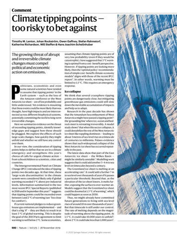
Environ Syst DecisTable 1 DICE base case results( are 200-year present values in2005 trillions)Emission tsMaximumtemperaturechange ( C)No controls 22.5 0 22.55.3Optimal controls 17.4 2.1 19.53.5L2.0C 13.4 11.8 25.22.0L1.5C 10.5 28.8 39.31.5that the input will fall above the value shown. As wedemonstrate below, these fractiles are useful in sensitivityanalysis.The CO2-ECS is uncertain because we are uncertainabout the ECS and the amount of forcing that will attend anincrease in CO2 concentrations. In characterizing ourunderstanding of the CO2-ECS, the IPCC (2007b) notesthatThe [CO2] equilibrium climate sensitivity is likelyto be between 2 C and 4.5 C, with a best estimateof 3 C and it is very unlikely to be less than 1.5 C.Values substantially higher than 4.5 C cannot beexcluded, but agreement of models with observationsis not as good for those values [emphasis in original].The IPCC defines likely as greater than a 66 % probability and very unlikely as less than a 10 % probability(IPCC 2005). Based on this, we assume that the CO2-ECSis lognormally distributed with a mean of 3.0 C andstandard deviation of 1.5 C. This distribution is shown inFig. 1. Compared to the normal distribution, assumed byNordhaus, the lognormal distribution is skewed to the rightand excludes the possibility of negative CO2 climate sensitivities (i.e., the addition of CO2 to the atmosphere willcool the Earth). With these assumptions, the P90 is veryclose to 1.5 C and there is about a 60 % chance of itsbeing between 2.0 and 4.5 C. The P90 is about 5.0 C, andthere is a 1 % chance that the climate sensitivity is above8.0 C. These ranges closely match the IPCC’s statementregarding uncertainty in the climate sensitivity.Since important DICE parameters are uncertain, so arethe maximum temperature change and the total costsincurred by following a particular emissions controlregime. Figure 2 shows the impact of input uncertainty ontotal costs under OC. This diagram, called a ‘‘tornadodiagram,’’ is centered at 19.5 trillion, which is the totalcost estimated by DICE when all input variables are set totheir base case and match the value given in Table 1.Figure 2 details the impact on total costs of varying oneinput at a time—holding the emissions reduction strategyconstant. For example, if the CO2-ECS was 5.0 C and allother variables were still at their base case, then total costswould be approximately 30 trillion. If the CO2-ECS was1.5 C and all other variables were at their base case, totalcosts would be approximately 10 trillion—a swing of 20trillion. Since there is an 80 % chance that CO2-ECS isbetween 1.5 and 5.0 C, there is an 80 % chance that totalcosts will be between 10 trillion and 30 trillion underOC, owing to uncertainty about the CO2-ECS alone.Similarly, there is an 80 % chance that total costs will bewithin the range shown for each of the other variables.Thus, we see that uncertainty in the CO2-ECS, the damageparameter, and the population, most contribute to ouruncertainty regarding total costs. The atmospheric retentionrate, the rate of decarbonization, the cost of the backstoptechnology, and the TFP growth rate contribute less to ouruncertainty regarding costs.It is important to stress that we are holding the emissionsreduction strategy constant. Thus, we do not allow societyto either act with perfect foresight (‘‘learn then act’’)Table 2 Key DICE uncertaintiesVariablesUnitsMeanStandard deviationP90P10CO2 equilibrium climate sensitivity C3.01.51.55.0Fraction of CO2 retained in atmosphere after 10 yearsFraction0.8110.0170.7890.8322Quadratic damage parameter trillions/( C)0.00280.00130.00120.0045Rate of growth in total-factor productivity%/year9.200.408.709.70Rate of decarbonization%/year-7.302.00-9.86-4.74Initial cost of backstop technologyAsymptotic global population 022123
Environ Syst Decis4 Reducing risk via emissions reductions0.40.350.3As discussed in the previous section, a handful of variables(those in Table 2) drive our uncertainty regarding temperature change and climate damages. In this section, weinvestigate how well one policy response, emissionreductions, lowers the risk of catastrophic damages.We begin by estimating the range within which themaximum temperature change could fall under each emissions control regime. We do this by performing a MonteCarlo simulation (10,000 trials) and sampling from theuncertainties in Table 2, again holding the emissions controlregime constant. The results appear in Fig. 4, which displaysthe probability of exceeding a particular temperature changeunder NC, OC, L2.0C, and L1.5C. Our uncertainty regardingtemperature changes is significant. For example, the maximum temperature change under NC could range from about1 C to 10 C. The mean or average maximum temperaturechange is 5.0 C. Under OC, this range is reduced somewhat, but temperature changes in excess of 7 or 8 C cannotbe ruled out. L1.5C and L2.0C shift the temperature distribution to the left, but even these tight emission controlregimes leave the possibility of exceeding 3 or 4 C.Figure 4 also shows the abatement cost required tomove between emission control regimes (as detailed inTable 1), thereby shift the temperature distribution to theleft. Moving from NC to OC incurs 2.1 trillion in abatement costs and shifts the temperature distribution to theleft, but a long tail remains. L2.0C costs 9.7 trillion morethan OC ( 11.8 trillion more than NC). We see that movingfrom OC to L2.0C has about the same effect on temperature as moving from NC to OC, but costs almost five timesa much. L1.5C costs 17 trillion more than L2.0C (about 29 trillion more than NC) and only slightly affects thetemperature distribution.Mean 1213CO2 Equilibrium Climate Sensitivity ( C)Fig. 1 Lognormal probability distribution for CO2 equilibriumclimate sensitivityregarding important uncertainties, such as the ECS, nor dowe allow for a dynamic strategy (‘‘learn, act, learn, act, ’’)where the emission control regime is adjusted as knowledgeof the climate system evolves. The former is clearly unrealistic and the later is structurally and computationallydifficult. For example, a dynamic strategy would requireone to model how our knowledge of key uncertainties couldchange over time and implement a stochastic decisionmaking algorithm (e.g., stochastic dynamic programming).An example of such a model can be found in Baranzini et al.(2003). We take a simpler approach here, with the hope thatour results will be more transparent and accessible.The sensitivity of the maximum temperature changeunder OC is shown in Fig. 3. Recall, the base case value is3.5 C (see Table 1). In this case, we see that the climatesensitivity dominates our uncertainty regarding temperature changes. The Earth’s population, the rate of decarbonizaiton of the world economy, and the retention rate ofatmospheric CO2 contribute much less to our uncertainty.The damage parameter and cost of the backstop technologyhave only a very minor impact.Fig. 2 Sensitivity of total costsunder optimal controlsPV Total Costs (trillions 2005 )Base Value 19.55.010.015.020.025.030.035.0Base ValueCO2 Equilibrium ClimateSensitivity ( C)Quadratic Damage Parameter( trillions / ( C)2)Asymptotic Population(millions)Atmospheric CO2 RetentionRateRate of Decarbonization(%/yr)Cost of Backstop Technology(000s 2005 /MTC)Annual TFP Growth 1,1709.2
Environ Syst DecisMaximum MeanTemperature Change ( C)Base Value 3.51.52.02.53.03.54.04.55.05.5Base ValueCO2Equilibrium ClimateSensitivity ( C))1.55.0Asymptotic Population(millions)6,17811,022Rate of Decarbonization(%/yr)-9.86AtmosphericCO2 RetentionRate0.789Annual TFP Growth Rate(%/yr)Quadratic Damage Parameter( trillions / ( C) 2 )-7.300.8320.0045Cost of Backstop Technology(000s 2005 01,769Probability of Exceeding TemperatureFig. 3 Sensitivity of maximum temperature change under optimal controls1.00Note: All dollars in trillions of 2005 0.900.80NC0.70L2.0COCL1.5C0.600.503.3ºC2.0ºCMean 5.0ºC0.401.5ºC0.300.20 17 9.7 2.10.100.00012345678910Temperature Change ( C)Fig. 4 Probability of exceeding particular temperatures under different emissions control regimesTable 3 details the probability of exceeding 2.0, 3.0, 4.0,or 5.0 C for the four emission control programs we consider. For example, OC produces an 85 % chance ofexceeding 2.0 C, a temperature change that scientists havewarned is dangerous. A deterministic emission controlpolicy designed to limit temperature change to 2.0 C stillhas about a 42 % chance of temperature change greaterthan 2.0 C. Even trying to limit temperature change to1.5 C runs almost a 20 % chance of exceeding a temperature change of 2.0 C.Similar results hold for more extreme temperaturechanges. Under NC, there is an 87 % chance of changegreater than 3 C. OC reduces this chance to 54 %. EvenL2.0C has an 11 % chance of change greater than 3 C;further tightening emission controls to hold temperaturechanges to 1.5 C reduces this chance to 3 %.We might also be concerned with the length of time weare above a threshold temperature, not simply whether ornot this threshold is crossed. Figure 5 displays the averagenumber of years that temperature changes exceeded thelisted values, under each emissions control scenario. UnderOC, the increase in the average temperature of the atmosphere exceeds 2 C for almost 120 years, on average, inour simulations. Under L2.0C, this is reduced to 60 years.Yet, these are average values. In 10 % of our scenarios, thetemperature increase under L2.0C exceeded 2 C for150 years. Thus, even strict emission control polices do notguarantee that the Earth will not exceed possibly dangerousthreshold temperatures for many decades, if not more thana century.It is disappointing that tight emission control regimesstill hold a non-negligible chance of exceeding a temperature threshold that scientists have suggested could lead tothe disintegration of the GIS. Thus, relying solely onemissions reductions to manage the risk of crossing tippingpoints could be risky. McInerney and Keller (2008) notethat reducing the odds of a collapse of the thermohalinecirculation (THC) to below 1-in-10 requires an almost‘‘complete decarbonization over the next 60 years.’’Reducing the odds to 1-in-100 reduces the timeframe toTable 3 Probability of exceeding particular temperatures under different emissions control regimesEmission control regimes2 C3 C4 C5 CNC0.980.870.670.45OCL
addressing climate tipping points via emissions reductions. In Sect. 5, we analyze the economic benefit of different CE policies and their ability to address climate tipping points. Rather than model uncertainty regarding the location and severity of climate tipping points, we consider many dif-ferent scenarios.