WIXLIB

NESUG 2010Health Care and Life SciencesSensitivity, Specificity, Accuracy, Associated Confidence Interval and ROCAnalysis with Practical SAS ImplementationsWen Zhu1, Nancy Zeng 2, Ning Wang 21K&L consulting services, Inc, Fort Washington, PA2Octagon Research Solutions, Wayne, PA1. INTRUDUCTIONDiagnosis tests include different kinds of information, such as medical tests (e.g. blood tests, X-rays, MRA), medicalsigns (clubbing of the fingers, a sign of lung disease), or symptoms (e.g. pain in a particular pattern). Doctor’sdecisions of medical treatment rely on diagnosis tests, which makes the accuracy of a diagnosis is essential inmedical care. Fortunately, the attributes of the diagnosis tests can be measured. For a given disease condition, thebest possible test can be chosen based on these attributes. Sensitivity, specificity and accuracy are widely usedstatistics to describe a diagnostic test. In particular, they are used to quantify how good and reliable a test is.Sensitivity evaluates how good the test is at detecting a positive disease. Specificity estimates how likely patientswithout disease can be correctly ruled out. ROC curve is a graphic presentation of the relationship between bothsensitivity and specificity and it helps to decide the optimal model through determining the best threshold for thediagnostic test. Accuracy measures how correct a diagnostic test identifies and excludes a given condition. Accuracyof a diagnostic test can be determined from sensitivity and specificity with the presence of prevalence. Given theimportance of these statistics in disease diagnosis and the terms are easily confused, it is important to get familiarwith how they work, it helps us better understand when to use, how to implement them, and how to interpret theresults. The importance and popularity of these statistics urges for a thorough review along with practical SASexamples.This paper will focus on the concepts of sensitivity, specificity and accuracy in the context of disease diagnosis:starting with a review of the definitions , how to calculate sensitivity, specificity and accuracy, associated 95%confidence interval and ROC analysis; followed by a practical example of disease diagnosis and related SAS macrocode; then moving on to the common issues on interpreting the results of sensitivity, specificity and accuracy; endedby a final remark of the entire paper.2. SENSITIVITY, SPECIFICITY AND ACCURACY, 95% CINFIDENCE INTERVAL AND ROCCURVE2.1 SENSITIVITY, SPECIFICITY AND ACCURACYOutcome of thediagnostic testPositiveCondition (e.g. Disease)As determined by the Standard of TruthNegativeRow TotalTP FPPositiveTPFP(Total number of subjects withpositive test)FN TNNegativeFNTN(Total number of subjects withnegative test)FP TNTP FNColumn total(Total number of subjectswith given condition)(Total number ofsubjects without givencondition)N TP TN FP FN(Total number of subjects instudy)Table 1. Terms used to define sensitivity, specificity and accuracyThe ideas described below are summarized in table 1.1

NESUG 2010Health Care and Life SciencesThere are several terms that are commonly used along with the description of sensitivity, specificity and accuracy.They are true positive (TP), true negative (TN), false negative (FN), and false positive (FP). If a disease is provenpresent in a patient, the given diagnostic test also indicates the presence of disease, the result of the diagnostic testis considered true positive. Similarly, if a disease is proven absent in a patient, the diagnostic test suggests thedisease is absent as well, the test result is true negative (TN). Both true positive and true negative suggest aconsistent result between the diagnostic test and the proven condition (also called standard of truth). However, nomedical test is perfect. If the diagnostic test indicates the presence of disease in a patient who actually has no suchdisease, the test result is false positive (FP). Similarly, if the result of the diagnosis test suggests that the disease isabsent for a patient with disease for sure, the test result is false negative (FN). Both false positive and false negativeindicate that the test results are opposite to the actual condition.Sensitivity, specificity and accuracy are described in terms of TP, TN, FN and FP.Sensitivity TP/(TP FN) (Number of true positive assessment)/(Number of all positive assessment)Specificity TN/(TN FP) (Number of true negative assessment)/(Number of all negative assessment)Accuracy (TN TP)/(TN TP FN FP) (Number of correct assessments)/Number of all assessments)As suggested by above equations, sensitivity is the proportion of true positives that are correctly identified by adiagnostic test. It shows how good the test is at detecting a disease. Specificity is the proportion of the true negativescorrectly identified by a diagnostic test. It suggests how good the test is at identifying normal (negative) condition.Accuracy is the proportion of true results, either true positive or true negative, in a population. It measures the degreeof veracity of a diagnostic test on a condition.The numerical values of sensitivity represents the probability of a diagnos tic test identifies patients who do in facthave the disease. The higher the numerical value of sensitivity, the less likely diagnos tic tes t returns false-positiveresults. For example, if sensitivity 99%, it means: when we conduct a diagnostic test on a patient with certaindisease, there is 99% of chance, this patient will be identified as positive. A test with high sensitivity tents to captureall possible positive conditions without missing anyone. Thus a test with high sensitivity is often used to screen fordisease.The numerical value of specificity represents the probability of a test diagnoses a particular disease without givingfalse-positive results. For example, if the specificity of a test is 99%. It means: when we conduct a diagnostic test ona patient without certain disease, there is 99% chance; this patient will be identified as negative.A test can be very specific without being sensitive, or it can be very sensitive without being specific. Both factors areequally important. A good test is a one has both high sensitivity and specificity. A good example of a test with highsensitive and specificity is pregnancy test. A positive result of pregnancy test almost for sure suggests the subjectwho took the test is pregnant. A negative result almost certainly rules out the possibility of being pregnant.In addition to the equation show above, accuracy can be determined from sensitivity and specificity, whereprevalence is known. Prevalence is the probability of disease in the population at a given time:Accuracy (sensitivity) (prevalence) (specificity) (1 - prevalence).The numerical value of accuracy represents the proportion of true positive results (both true positive and truenegative) in the selected population. An accuracy of 99% of times the test result is accurate, regardless positive ornegative. This stays correct for most of the cases. However, it worth mentioning, the equation of accuracy impliesthat even if both sensitivity and specificity are high, say 99%, it does not suggest that the accuracy of the test isequally high as well. In addition to sensitivity and specificity, the accuracy is also determined by how common thedisease in the selected population. A diagnosis for rare conditions in the population of interest may result in highsensitivity and specificity, but low accuracy. Accuracy needs to be interpreted cautiously.2.2 ASYMPTOTIC AND EXACT 95% CONFIDENCE INTERVALThe sensitivity, specificity and accuracy are proportions, thus the according confidence intervals can be calculated byusing standard methods for proportions 1. Two types of 95% confidence intervals are generally constructed aroundproportions: asymptotic and exact 95% confidence interval. The exact confidence interval is constructed by usingbinomial distribution to reach an exact estimate. Asymptotic confidence interval is calculated by assuming a normalapproximation of the sampling distribution. The choice of these two types of confidence interval depends on whetherthe sample proportion is a good approximation of normal distribution. If the number of event is very small or if thesample size is very small, the normal assumption cannot be met. Thus, exact confident interval is desired. SASexample for both types of 95% confidence intervals will be provided in section 3.2

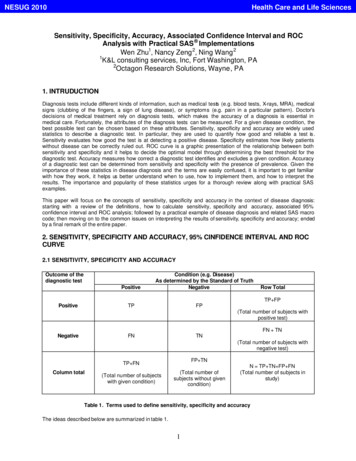
NESUG 2010Health Care and Life Sciences2.3 RECEIVER OPERATING CHARACTERISTICS (ROC) ANALYSISFor a given diagnostic test, the true positive rate (TPR) against false positive rate (FPR) can be measured, whereTPR TP/(TP FN)AndFPR FP/(FP TN)As we can see from the above equations, TPR is equivalent to sensitivity and FPR is equivalent to (1 – specificity). Allpossible combinations of TPR and FPR compose a ROC space. One TPR and one FPR together determine a singlepoint in the ROC space, and the position of a point in the ROC space shows the tradeoff between sensitivity andspecificity, i.e. the increase in sensitivity is accompanied by a decrease in specificity. Thus the location of the point inthe ROC space depicts whether the diagnostic classification is good or not. In an ideal situation, a point determinedby both TPR and FPF yields a coordinates (0, 1), or we can say that this point falls on the upper left corner of theROC space. This idea point indicates the diagnostic test has a sensitivity of 100% and specificity of 100%. It is alsocalled perfect classification. Diagnostic test with 50% sensitivity and 50% specificity can be visualized on the diagonaldetermined by coordinate (0, 0) and coordinates (1, 0). Theoretically, a random guess would give a point along thisdiagonal. A point predicted by a diagnostic test fall into the area above the diagonal represents a good diagnosticclassification, otherwise a bad prediction. A graphic presentation of what described above is shown in figure 1.1Ideal coordinate (0, 1)0.8Cut-point0.6Sensitivity (TPR)Random classification0.40.200.20.40.60.811-specificity (FPR)Figure 1: ROC Space: shadow area represents better diagnosticclassificationA single cut-point of a diagnostic test defines one single point in the ROC space; however, different possible cutpoints of a diagnostic test determine a curve in ROC space, which is also called ROC curve. Like a single point in the3