Transcription
A NEW TIME DOMAIN WAVEFORM MEASUREMENT SETUPTO INVESTIGATE INTERNAL NODE VOLTAGES IN MMICs.Tibault Reveyrand(1), Alain Mallet(1), Francis Gizard(1), Luc Lapierre(1),Jean-Michel Nébus(2), Marc Vanden Bossche(3)(1)CNES – DCS/RF/HT18, Avenue Edouard Belin31401 Toulouse Cedex 9 - FranceEmail: alain.mallet@cnes.fr(2)IRCOM123, Avenue Albert Thomas87060 Limoges Cedex - FranceEmail: nebus@ircom.unilim.fr(3)NMDG EngineeringFountain Business Center, Building 5, Cesar van Kerckhovenstrat 110B-2880 Bornem - BelgiumEmail: marc.vanden bossche@nmdg.beINTRODUCTIONTime domain waveforms engineering at internal nodes of MMICs is essential for the phenomenologic understanding ofthe nonlinear elements behavior inside of MMICs. This topic is extremely enriching in various fields as varied as thecircuits reliability, the nonlinear parmetric stability and, in a general way, the optimal design and behavior survey ofMMICs.This approach, usually performed in simulation, is possible henceforth in instrumentation and characterization. Thedescription of the measurement setup and the calibration procedure is the object of this paper.The heart of the measurement setup have to be an instrument which provide the capabilities to measure RF multiharmonics time domain waveforms. The ‘Large Signal Network Analyser’ (LSNA) is a perfect solution to perform thiskind of measurements. It enables time domain waveform measurements of a device under test, provides a NISTvalidated calibration (specilly a phase calibration) procedure and is commercially available through ‘MauryMicrowave’.This paper presents a way to modify the classical LSNA system and its calibration procedure in order to enable timedomain waveforms at internal nodes of MMICs with high impedance probes (HIP). The HIP calibration andmeasurement procedures can be easily added to the original LSNA driver software. Indead, the HIPs are considered likea classical test-set through the software and do not modify the traditionnal use of the LSNA.This work is applicated here to the characterization of a class-F amplifier at S band.THE LARGE SIGNAL NETWORK ANALYSER (LSNA) [1]The LSNA could be seen as a vectorial network analyser (VNA) enhanced to nonlinear devices characterization. Thewaves (incident / reflected waves or voltages and currents) are measured in an absolute way : the LSNA enables wavesmagnitudes and phases measurements (and not ratios only like with VNAs) and performs measurements at differentsfrequencies simultaneously (a CW fundamental and all harmonics).The characterization tool [2]The LSNA hardware architecture is very close from the VNA one. The main difference is the receiver part(downconverter process) : a sampling convertor take the place of the classical mixer. The sampling rate is around 20MHz and leads to a signal frequency-compressed within a 10 MHz bandwidth. This low-frequency downconvertedsignal is sampled with ADC.
10 MHzATTIFSource«RACK VXI »AATTATT« DOWN-CONVERTERBOX »ADCAATTADCAADCADCAClock« TEST-SET »DSTRF SourceMatch(50 Ohms)Fig. 1. LSNA : the simplified architectureThe calibration procedure [3]The calibration error-model of the LSNA is defined as a 8-terms matrix. 7 of thoses 8 terms are known by a classicalVNA relative calibration (SOLT or LRRM). The last (8th) term defines the absolute calibration in order to measureaccuratly both amplitude and phase of a single travelling wave. This term is calculated from a calibration with anamplitude standard (powermeter) and a phase standard (the harmonic phase reference : HPR). The relationship betweenthe non-corrected raw-data (ri) and the real physical travelling waves at the reference plane (ai and bi) can be written asthe 8-term following matrix :00 r1 1 βI a1 00 r2 j.ϕ{K } γ I δ I b1 (1) K .e a 0 0 α II β II r3 2 b 0 0 γ II δ II r 4 2 DUTThe LSNA calibration procedure is proceed in 3 steps :- A classical VNA relative calibration to define 7 of the 8 errors terms ;- An amplitude calibration by measuring a forward waveform with both the LSNA and a powermeter to define themagnitude of the 8th error term ;- A phase calibration by connecting the reference phase generator at a port of the LSNA to deduce the phasecorrection of the 8th error term.Then, the complete calibration matrix is computed as follow : α1CAL β1CAL v1 00 r1 CALCAL00 r2 γ1δ1 i1 (2) v2 r3 00α CALβ CAL22 i2 0γ CALδ CAL r 4 LSNA LSNA 022The phase standard (HPR) is a step recovery diode (SRD). It generates a very stable pulse. This pulse contains a lotof frequencies. The phase relationship between these frequencies has been precharacterize either with a RF scopecalibrated with the ‘nose to nose’ technique [3] (the Agilent’s method) or with a electro-optic sampling system [4] (theNIST’s method).ABOUT THE USE OF HIGH IMPEDANCE PROBES (HIP)Basic considerationsAs it has been shown in the calibration matrix expression, the corrected quantities which are measured by the LSNA arethe voltage v and current i. These terms are deduced from the voltage traveling waves (or voltage normalized pseudo-
waves) a and b such as : v a b a V a b(3) (4)andwith Z0 50 ohms i b V Z0We are going to use the same formalism about the high impedance probe in order to deduce the pseudo-wave a and bfrom the corrected measured voltage v. With this approach, Z0 is the caracteristic impedance of the probed line and thuscould include an imaginary part at low frequencies [5].According to the telegraphists equations, the incident (a or V ) and reflected (b or V-) pseudo-waves can be deducedfrom 2 simultaneous voltage measurements (v1 and v2) on a lonely probed propagation line as follow : v1 .e γ.L v 2 V 2.Sinh (γ.L )(5) γ .L v2v V 1 .e 2.Sinh (γ.L )where γ is the propagation constant of the propagation line and L the distance between the two probing locations.Thus, we need the propagation constant of the probed line (γ) to obtain the voltage travelling waves and both thepropagation constant and the characteristic impedance (Z0) to calculate the current travelling waves.Previous works about HIPsThe first works about this topic have been realized by J.C.M. Hwang from the Lehigh university. He has used for thatpurpose a Microwave Transcient Analyser (MTA) [6] [7] [8]. The results have illutrated the great interest of this kind ofmeasurement setup but the calibration procedure was not fully described. Indead, the high impedance probe have to bepreliminary characterized. The MTA is not a fully calibrated mesurement instrument and introduces phase distortionwhich is neglected but not negligible [2].In [9], U. Arz describes a classical and a new optimized method to get the S-parameters of a HIP with a VNA. Those Sparameters provide a practical mean for correcting raw measurements. In [10], P. Kabos illustrates and validatescalibrated time-domain oscilloscope measurements using these previous HIP S-parameters. He comes to the followingexpression :V (f ) VOSC (f ).[K (f )](6)1 S 22 (f ).Γ(f )1 S 22 (f ).Γ(f )with K (f ) S 21 (f ).Γ(f ) S11 (f ).(7)S 21S 21V(f) is the corrected voltage at the tip of the HIP. K(f) define a voltage transfert function of the HIP. Γ(f) is thereflexion coefficient of the scope and the S parameters are the HIP’s ones.At last, theses methods (with the MTA or the scope) are complex and require several measurements and connections /disconnections. The LSNA architecture enables more flexibility with the use of HIP. Then it becomes very easy todetermine the value of K(f) in (6).THE NEW SETUP AND ITS CALIBRATION PROCEDURESOur measurement setup use the LSNA in a « receiver mode » like. Two HIPs are connected to 2 receiver channels ofthe LSNA and are similar to a lumped reflectometer. This is the port 1 of our new test-set located into the device undertest. The port 2 use the classical test-set (reflectometer) to perform measurements at the output of the circuit.To calibrate this new measurement setup, we just have to use the LSNA standard calibration code to generate a 8-termscalibration matrix and then to swap the 4-error terms relatives to the ‘port 1’ with the new ones relatives to the HIPs. Anew ‘Mathematica’ module, developped for this new approach, performs this tranformation automatically : finally, theuser drives the measurement setup like a classical LSNA.The calibration procedure is performed in 3 steps.The first step consists in calibrating the LSNA with a probe station in a classical way (LRRM process, powermeter andHPR). This procedure generates the complete 8-terms calibration matrix. Then, we disconnect the input channels 1 and2 of the downconverter box from the test-set and connect the HIPs as illustrated figure 2. The port 2 is calibrated yet,and will be consider as our new voltage (or current) standard in order to calibrate high impedance probes.
The second step consists in probing sequentially the thru line of the calibration kit with the HIPs at the port 2 referenceplane. Then we can calculate the ratio of 2 measurements : v2 (the error corrected measurements provided by port 2)and r1 or r2 (the down-converted raw data corresponding to the probing HIPs). This ratio (calculated in the frequencydomain for each frequency of a sweep-sin) looks like K(f) in (6) ; but here, the voltage transfert function describe notonly the HIP but also a bias tee (placed between the HIP and the down-converter box to protect the sampling convertorfrom continuous current within disable DC measurements) and the downconverter hardware in the receiver :v2(f )v2(f ) K 1 (f ) and K 2 (f ) (8)r1(f )r 2(f )The third step is the generation of a new calibration sub-matrix associated to the port 1 of the test-set as follow : v1 α 1HIP β1HIP r1 HIP(9) δ1HIP r 2 i1 γ 1We have to calculate 4 terms and include this sub-matrix in the whole system calibration matrix as illustrated in figure2.Figure 2 shows the final measurement setup. r1 and r2 are the uncorrected raw data coming from the high impedanceprobes. r3 and r4 are the raw data from port 2. v2 and i2 are the corrected measurements at the calibrated port 2reference plane (tip of the GSG probe). v1 and i1 are deduced from r1 and r2 and represent the physical quantities at thetip of one high impedance probe.{r1 ; r2}1DOWN-CONVERTERBOX2 α1HIP v1 i1 γ 1HIP v 2 0 i2 LSNA 0β1HIPδ0 r1 0 r2 CAL r3 β2 δ 2CAL r 4 LSNA0HIP100α 2CAL0γ 2CAL{r3 ; r4}34TEST-SETA1A250ΩB150ΩB212HIP1HIP2GSGGSG{v1 ; i1}{v2 ; i2}Fig. 2. LSNA associated with HIPs : the measurement setup. The port 2 is used in a traditional way.The port 1 is used s a “receiver mode”.40180359030025-9020Argument (degree)Magnitude (dB)There are 3 differents methods to calculate the port 1 calibration sub-matrix. The 2 first methods use as an assumptionthe relation (6). A third method don’t need any assumption but require accurate values of the propagation constant andthe caracteristic impedance of the probed line even to deduce a single voltage value.Figure 3 illustrate K(f) (the HIP voltage transfert function versus the frequency) obtained at the second calibration step.This information is essential to build the calibration sub-matrix at the third step by using one of the 2 first methods.-180123456789 10 11 12 13 14 15 16 17 18 19 20Frequency (GHz)Fig. 3. Magnitude and phase of K(f) : the voltage transfert function between the tip of one high impedance probe andthe associated raw data.
Method 1This method is an easy way to enable 2 simultaneously corrected voltage measurements with HIPs. This methodconsists on the use of K1 and K2 (the pre-characterizated ratio of 2 HIPs) to define the matrix (9) : v1 K 1 0 r1 (10) i1 0 K 2 r 2 With this new calibration sub-matrix, we can obtain the voltage at the tips of both HIP but not the currents. Thus, in theLSNA software, the i1 waveform is not the current but the voltage at the tip of the second HIP. This method has to beused when we require independents HIPs.Method 2Some applications require the measurement of the current. Then, a second possibility has been implemented in thesoftware to fix the errors terms consequently. According to the telegraphists equations, the user have to know thedistance between the 2 HIPs, the propagation constant of the probed line (γ) and its characteristic impedance (ZC). K10 v1 r1 K 1 .Coth (γ.L ) K2(11) r 2 i1 (γ)ZC Z C .Sinh .L But the use of the K(f) ratio cancel any coupling effect between the 2 HIPs because the calculated β1HIP in (9) is nullwith this method. To take into account this coupling effect, we have to proceed to a new second step in the calibrationprocedure and define a sub-matrix instead of a single K(f) ratio.Method 3 : Calibration of coupled HIPsThis method don’t use any assumption about a K(f) voltage ratio. The calibration of the high impedance probes has tobe done with 2 HIPs simultaneously on a transmission line. One of the HIPs has to be placed at the port 2 referenceplane (standard of our HIP calibration). The aim of the calibration, with this method, is to deduce the complete 4-termserrors matrix (9) instead of the K(f) ratio (8).To find out the 4 errors terms associated to the HIPs, we have to solve 2 equations with 4 unknown factors, so we need2 different voltage/current standards. It’s possible by removing the classical 50 ohms termination at the output of thetest set (port ‘RF IN 2’) with an ‘Open’ or a ‘Short’. The corresponding modified voltage and current standards aremeasured at the reference plane with the calibrated port 2. This procedure provides additive measurement necessary todetermine the 4-terms error matrix relative to the HIPs. Here come the calibration sub-matrix : r 2 C 2 .v2 C1 r 2 C1.v2 C 2 r1C 2 .v2 C1 r1C1.v2 C 2 v1 r1C1.r 2 C 2 r1C 2 .r 2 C1 r1C 2 .r 2 C1 r1C1.r 2 C 2 r1 (12) i1 r 2 C 2 .i 2 C1 r 2 C1.i 2 C 2 r1C 2 .i 2 C1 r1C1.i 2 C 2 r 2 r1C1.r 2 C 2 r1C 2 .r 2 C1 r1C 2 .r 2 C1 r1C1.r 2 C 2 where the subscripts C1 and C2 indicate the condition of measurements (‘Open’ or ‘Short’ at the output of the test-set)for both the raw data (r1 and r2) and the standards at the GSG tip reference plane (indeed, the corrected measurementsv2 and i2).During the measurements, the distance between HIPs, the propagation constant and the characteristic impedance mustbe equal to the ones used (but unknown) during calibration.This restriction implies that we have to use the same substrate during calibration and measurements.Method 3 : Measuring on a substrate different from the calibration oneTo proceed a HIP calibration on a substrat and perform some measurements on another substrate, we need to know allthe characteristic parameters during the calibration and the measurements which are the propagation constants, thecharacteristic impedances and the distances between HIP of both substrates. Then, according to the telegraphistsequations and assuming that 2 HIPs behave like a lumped-reflectometer with 4 wave-coupling factors as illustatedfigure 4, we can create a new sub-matrix error from the one obtained during the calibration procedure and thecharacteristic parameters values by extracting theses 4 coupling factors values.We can deduce a new calibration sub-matrix correspounding to a measurement substrate (subsripted ‘MEA’) from thecomplete calibration sub-matrix (9) identified with the calibration substrate (subsripted ‘CAL’) and the physicalparameters of both substrats (the distance between the 2 probe locations, the propagation constant γ and the caracteristicimpedance ZC) :
α1HIPNEW Sinh (γ CAL .L CAL ). α1HIP .Cosh ((γ CAL .L CAL ) (γ MEA .L MEA )) Z C CAL .γ1HIP .Sinh ((γ CAL .L CAL ) (γ MEA .L MEA ))Sinh (γ MEA .L MEA )[(HIPβ1HIPNEW β1 .γ 1HIPNEW )]) (Sinh (γ CAL .L CAL )Sinh (γ MEA .L MEA )(13)(14)Sinh (γ CAL .L CAL )1. Z C CAL .γ1HIP .Cosh ((γ CAL .L CAL ) (γ MEA .L MEA )) α1HIP .Sinh ((γ CAL .L CAL ) (γ MEA .L MEA ))Z C MEA Sinh (γ MEA .L MEA )HIPδ1HIPNEW δ1 .[()]) (ZC CAL Sinh(γ CAL .L CAL ).Z C MEA Sinh (γ MEA .L MEA )(15)(16)Method #2Calibration HIPK1 HIPK1Method #3SIGNAL Analysis K1 HIPMeasureHIPHIP K2NETWORK Analysis K 2 K1 K1 K 2NETWORK AnalysisHIPHIP K 2 K1 K 2NETWORK AnalysisFig. 4. Calibration and measurements with methods 2 and 3. Method 2 does not take into account the coupling effectbetween the 2 HIPs : the incident ( ) and reflected (-) waves have the same transfert function.CALIBRATION COMPARISON (GSG AND HIP)The method number one has been used, first to measure the voltage along a line and secondly to test the design of apower amplifier.Several voltage measurements have been made on a 50Ω line during a ‘sweep-sin’ excitation (different power levelsand frequencies of the RF source). Figure 5 shows the voltage measured with a calibrated GSG probe (conventional useof the LSNA) and with a calibrated HIP on a propagation line which not use during the calibration. The comparison isquite good.310,7521,50,510,25Magnitude (volt)Argument (rad)2,50,50012345678910 11 12 13 14 15 16 17 18 19 20Frequency (GHz)Fig. 5. Calibrated voltage measurements at the tip of a GSG probe and a HIP during a sweep-sin.APPLICATION TO THE CHARACTERIZATION OF A CLASS-F POWER AMPLIFIERA class-F power amplifier has been measured. Basically, an optimized class-F amplifier have to present a squarevoltage waveform at the output of the transistors but not necessarily at the output of the amplifier because of thefiltering effects of the matching and the power combining networks. Internal waveform probing is the lonelyexperimental way to check the pertinent and successful design and realization of such topology.
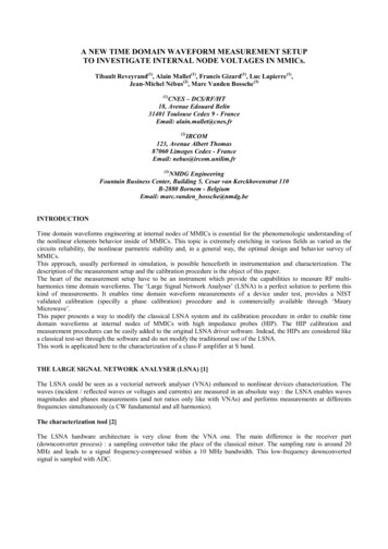
The device under testThe device under test is a MMIC S-band one-stage power amplifier. The circuit is built in HBT technology. Design goalwas to produce an optimized class F for a fundamental frequency equal to 2.15 GHz [11]. The bias are Vbe0 1 voltsand Vce0 9 volts. Because of the class F, the expected efficiencies of the transistor are about 70%.We probed the voltage at differents location on the MMIC for several input power. Figures 6 to 8 illustrate themeasurements results. The time domain waveforms are displayed upon 930 ps (2 fundamental periods).Measurement Results8866420-2-4-6-8Fig. 6. Calibrated voltage measurements at the outputof the MMIC.VHIP calibrated (Volt)VLSNA calibrated (Volt)1010420-2-4-6-8-10Fig. 8. Calibrated voltage measurements at the outputof a HBT.1,51VHIP calibrated (Volt)0,50-0,5-1-1,5-2-2,5-3Fig. 7. Calibrated voltage measurements at the input ofa HBT.Fig. 9. Picture of the MMIC during measurements.Figure 9 shows a picture of the experiment. We have used one dual positioner (FPD 100 : Fine-Pitch Dual Positioner) tohandle 2 high impedance probes (Cascade FPS-20X : Fine Pitch Signal) [12]. The probes are not connected to theground, neither during calibration nor measurements [9].The output of the MMIC has been measured with both a GSG probe (LSNA’s port 2) and a calibrated HIP. The timedomain waveforms are strictely the sames. The measurements at the input of the transistors lead to typical waveforms.At high input power, we can see a quasi-square voltage waveform at the output of each transistor which validate thedesign topology and method for this class-F amplifier demonstrator.CONCLUSIONHigh impedance probe calibrations and measurements procedures have been described and implemented in the LSNAsoftware (a single ‘Mathematica’ module). This module has to be linked to the original ‘Mathematica’ kernel of theLSNA driver. This tool provides a friendly and easy way to investigate waveforms at internal nodes of MMICs.An application has been presented concerning the validation of an high efficiency amplifier design. This measurementsystem is expected to be essential for the stability analysis of MMIC because it offers an unique experimentalverification of even and odd ocillation modes [13].As a conclusion, the use of the LSNA with HIPs strongly reinforces the links needed between the measurement and thesimulation environments. It enables a better understanding of nonlinear effects and contributes to improved optimizeddesigns of reliable MMICs.
ACKNOWLEDGEMENTSThe authors gratefully acknowledge NMDG Engineering for the loan of the complete LSNA system, CascadeMicrotech for the loan of two high impedance probes and their 10][11][12][13]Maury Microwave, “Large-Signal Network Analyser, Bringing Reality To Waveform Engineering”, technicalData Sheet 4T-090 rev A, june 2003, http://www.maurymw.comE. Vandamme, J. Verspecht, F. Verbeyst and M. Vanden Bosshe, “Large Signal Network Analysis – ameasurement concept to characterize nonlinear devices and systems”, Application Note, Agilent Technologies,Inc. , June 2002.J. Verspecht, “Calibration of a measurement system for high frequency nonlinear devices”, Ph.D. dissertation,Vrije Univ., Brussels, Belgium, Nov. 1995.D.F. Williams, P.D. Hale, T.S. Clement, and J.M. Morgan., “Calibrating Electro-Optic Sampling Systems”,IEEE MTT-S, Phoenix, AZ, pp. 1527-1530, May 20-25, 2001R.B. Marks, D.F. Williams, “A General Circuit Waveguide Theory”, Journal of Research of the NationalInstitute of Standards and Technology, vol. 97, n 5, pp. 533-562, September-October 1992.C.J. Wei, Y.A. Tkachenko and J.C.M.Hwang, “Non-invasive waveform probing for nonlinear network analysis”,IEEE MTT-S Digest 1993C.J. Wei, Y.A. Tkachenko, J.C.M. Hwang, K.R. Smith and A.H. Peake, “Internal-Node Waveform Analysis ofMMIC Power Amplifier”, IEEE Trans. On MTT, vol.43, n 12, dec 1995, pp. 3037-3042J.C.M. Hwang, “Internal Waveform Probing of HBT and HEMT MMIC Power Amplifiers”, 60th ARFTGConference Digest, Fall 2002, December 5th & 6th 2002, Washington DC, pp.111-112U. Arz, H.C. Reader, P. Kabos, and D.F. Williams, “Wideband frequency-domain characterization of highimpedance probes”, 58th ARFTG Conference Digest, San Diego, CA, USA, November 2001P. Kabos, H.C. Reader, U. Arz, and D.F. Williams, “Calibrated Waveform Measurement with High impedanceProbes”, Trans. on MTT, vol.51, n 2, February 2003,pp. 1095-1098A. Mallet, T. Peretallade, R. Sommet, D. Floriot, S. Delage, J.M. Nébus and J. Obregon “A design methode forhigh efficiency class F HBT amplifiers”, IEEE MTT-S 96, san Fransisco, CA, june 17-21, 1996, ww.cascademicrotech.comA. Anakabe, J. M. Collantes, J. Portilla, J. Jugo, A. Mallet, L. Lapierre, J.P. Fraysse, “Analysis and Eliminationof Parametric Oscillations in Monolithic Power Amplifiers”, IEEE MTT-S Digest, pp. 2181-2184, 2002
validated calibration (specilly a phase calibration) procedure and is commercially available through 'Maury Microwave'. This paper presents a way to modify the classical LSNA system and its calibration procedure in order to enable time domain waveforms at internal nodes of MMICs with high impedance probes (HIP). The HIP calibration and