WIXLIB

IMutation–selection modelsThis chapter and the following are concerned with models for mutation and selection, inwhich effects of other evolutionary forces are neglected. These models are introduced inSection 1 on a general basis. Afterwards, for the rest of this chapter, we restrict ourselvesto the case that individuals are characterized by genotypes from a large but finite set.Section 2 introduces the specific model under consideration and connects it to a multitypebranching process, both forward and backward in time. The latter direction gives rise tothe definition of the distribution of ancestors, which will play an important role in thesequel. In Section 3, the main results, which allow for a simple characterization of theequilibrium population, are formulated, proved, and discussed. As an application, Section4 treats threshold phenomena that may occur when the mutation rates are varied, suchas the well-known error threshold. Chapter II is then devoted to so-called continuumof-alleles (COA) models, in which the genotypes are characterized by the elements ofa continuous set, such as R or the interval [0, 1]. As a general reference for mutation–selection models, Bürger’s book [Bür00] is recommended.1The general modelWe consider the evolution of an effectively infinite population of haploid1 individualssubject to mutation and selection. Disregarding environmental effects, we take individualsto be fully described by their genotypes, which are labeled by the elements of some setΓ endowed with a positive σ-finite measure ν (usually the Haar measure). This set mayeither be finite, Γ {1, . . . , M }, with ν being the counting measure, or an intervalΓ R equipped with the Lebesgue measure. The set Γ may be taken either as thewhole genome, or as the genomic basis of a specific trait or function (i.e., an observablephenotypical property). We will describe the population at time t byRa probability densityon Γ , i.e., an integrable function p(t) L1 (Γ, ν) with p(t) 0 and Γ p(x, t) dν(x) 1.2Throughout this and the following chapter, we will use the formalism for overlappinggenerations, which works in continuous time, and only comment on extensions to theanalogous model for subsequent generations in discrete time. The standard equationthat describes the evolution of the density p(t) is, cf. [Kim65] and [Bür00, (IV.1.3)],Z¡ ¡ u(x, y) p(y, t) u(y, x) p(x, t) dν(y) .(1)ṗ(x, t) r(x) r̄(t) p(x, t) Γ1Diploid individuals without dominance may be described by the same formalism since the reproduction rate of an allele combination is additive with respect to both alleles, compare [Bür00, Sec. III.2.1].2For a treatment of the general case of arbitrary locally compact spaces Γ and the description interms of probability measures, see [Bür00, Sec. IV].1

I. MUTATION–SELECTION MODELSHere, r(x) is the Malthusian fitness, or (effective) reproduction rate, of type x Γ ,which isR connected to the respective birth and death rates as r(x) b(x) d(x), andr̄(t) Γ r(x) p(x, t) dν(x) designates the mean fitness. The mutation rates and thedistributions of mutant types are given by u, where u(x, y) corresponds to a mutationfrom type y to x, and the dot denotes the time derivative / t.In this model, mutation and selection are assumed to be independent processes, goingon in parallel. However, mutation may also be viewed as occuring during reproduction.In this case, we have u(x, y) v(x, y) b(y), where v(x, y) gives the respective mutationprobability during a reproduction event and the distribution of mutants. Since, formally,this leads to the same type of model, it will not be discussed separately.2The model with discrete genotypes2.1Deterministic descriptionLet us, for the rest of this chapter, turn exclusively to the model with discrete genotypes,for which Γ {1, . . . , M }. Here, we identify the population density p(t) with a vectorp(t) (pi (t))1 i M , which reflects the canonical coordinatization. The evolution equation(1) becomes the following system of ordinary differential equations, cf. [Cro70, Hof85],X¡¡ ṗi (t) Ri R̄(t) pi (t) mij pj (t) mji pi (t) .(2)jFor reasons that will become clear in Section 2.6, we use capital letters for the reproduction rates Ri here. Further, we write mij for the mutation rate from type j to i.3For some of the main results of this chapter, further assumptions on the mutationscheme are required. To this end, we collect genotypes into classes Xk of equal fitness,0 k N , and assume mutations only to occur between neighboring classes. Let Rkdenote the fitness of class k and Uk the mutation rate from class Xk to Xk 1 (i.e., the totalrate for each genotype in Xk to mutate to some genotype in Xk 1 ), with the conventionU0 UN 0. Thus, we obtain a variant of the so-called single-step mutation model,¡ ṗk (t) Rk R̄(t) Uk Uk pk (t) Uk 1pk 1 (t) Uk 1pk 1 (t) .(3)(Here, the convention p 1 (t) pN 1 (t) 0 is used.) We can, for example, think of X0as the (mutation-free) wildtype class with maximum fitness and fitness only dependingon the number of mutations carried by an individual. If, further, mutation is modeledas a continuous process (or if multiple mutations during reproduction can be ignored),Equation (2) reduces to (3), with an appropriate choice of mutation classes. Dependingon the realization one has in mind, the Uk then describe the total mutation rate affectingthe whole genome or just the trait or function under consideration.In most of our examples, we will use the Hamming graph as our genotype space. Here,genotypes are represented as binary sequences s s1 s2 . . . sN { , }N , hence M 2N .3Generally throughout this thesis, I use this index convention, which is the transposed of what iscommon for Markov processes but more natural in the context of differential equations.2

2. THE MODEL WITH DISCRETE GENOTYPES (1 κ)µ(1 κ)µ Figure 1: Rates for mutations and back mutations at each site or locus of a biallelic sequence.The two possible values at each site, and , may be understood either in a molecularcontext as nucleotides (purines and pyrimidines) or, on a coarser level, as wildtype andmutant alleles of a biallelic multilocus model. We will assume equal mutation rates atall sites, but allow for different rates, (1 κ)µ and (1 κ)µ, for mutations from to and for back mutations, respectively, according to the scheme depicted in Figure 1. Here,µ 0 describes the overall mutation rate and κ [ 1, 1] is an asymmetry parameter.Clearly, the biallelic model reduces to a single-step mutation model (with the sameN ) if the fitness landscape4 is invariant under permutation of sites. To this end, wedistinguish a reference genotype s . . . , in most cases the wildtype, and assumethat the fitness Rs of sequence s depends only on the Hamming distance k dH (s, s )to s (i.e., the number of mutations, or ‘ ’ signs in the sequence). The resulting totalmutation rates between the Hamming classes Xk and Xk 1 readUk (1 κ) µ (N k) and Uk (1 κ) µ k(4)if mutation is assumed to be an independent process at all sites. We usually have thesituation in mind in which fitness decreases with k and will therefore speak of Uk andUk as the deleterious and advantageous mutation rates. However, monotonic fitness isnever assumed, unless this is stated explicitly.In much of the following, we will treat the general model (2), which builds on singlegenotypes, and the single-step mutation model (3), in which the units are genotypeclasses, with the help of a common formalism. To this end, note that both models can berecast into the following general form using matrices of dimension M , respectively N 1:¡ ṗ(t) H R̄(t)1 p(t) .(5)Here, 1 is the identity. The matrix H R M is composed of a diagonal matrix Rthat holds the Malthusian fitness values, and the mutation matrix M (Mij ) with eitheroff-diagonal entries reading mij , orPwith Uk on the secondary diagonals. The diagonalelements in each case are Mii j6 i Mji , hence the column sums vanish, i.e., M is aMarkov generator. Where the more restrictive form of the single-step model is needed,this will be stated explicitly. Unless we talk about unidirectional mutation (Uk 0 forthe single-step mutation model), we will always assume that M is irreducible (i.e., eachentry is non-zero for a suitable power of M ).Let now T (t) : exp(tH), with matrix elements Tij (t). Then, the solution of (5) isgiven by (see, e.g., [Bür00, Sec. III.1])p(t) PT (t)p(0),i,j Tij (t)pj (0)(6)4We use the notion of a fitness landscape [Kau87] as synonymous with fitness function for the mappingfrom genotypes to individual fitness values.3

I. MUTATION–SELECTION MODELSPPas can easily be established by using i,j Hij pj (t) i Ri pi (t) R̄(t) and differentiating.5 Due to the irreducibility, the population vector converges to a unique, globallystable equilibrium distribution p : limt p(t) with pi 0 for all i, which describesmutation–selection balance (cf., e.g., [Bür00, Sec. IV.2]). By the Perron–Frobenius theorem (compare [Sch74, Sec. I.6] or [Gan86, Sec. 13.2]), p is the (right) eigenvector corresponding to the largest eigenvalue, λmax , of H. (Strictly speaking, if there are negativefitness values, we have to add a suitable constant C to all fitness values to make H positive, i.e., all its entries non-negative. Then, λmax is given by the spectral radius of H C,which is its largest eigenvalue, minus C.) For unidirectional mutation, the equilibriumdistribution p is in general not unique, see the discussion in Section 3.2.2.2The corresponding branching processOur approach will heavily rely on genealogical relationships, which contain more detailedinformation than the time evolution of the relative frequencies (6) alone. On the nextpages, we therefore reconsider the mutation–selection model as a branching process.6We consider the process of mutation, reproduction and death as a (continuous-time)multitype branching process, as described previously for the discrete-time variant of theso-called quasispecies model, i.e., the analogous model with mutation coupled to reproduction [Dem85, Hof88, Ch. 11.5]. Let us start with a finite population of individuals,each described by an element i of a finite set Γ , that reproduce (at rates Bi ), die (at ratesDi ), or change type (at rates Mij ) independently of each other, without any restrictionon population size. Let Yi (t) be the random variable denoting the number of individualsof type i at time t, and ni (t) the corresponding realization; collect the components intovectors Y, n N0 Γ , and let¡ ei be the i-th unit vector. The transition probabilitiesfor¡ the joint distribution,PrY (t) n(t) Y (0) n(0) , which we will abbreviate as Pr n(t) n(0) by abuse of notation, are governed by the differential equation7X ¡ ¡Xd ¡Pr n(t) n(0) (Bi Di Mji ) ni (t) Pr n(t) n(0)dtij6 iX ¡ ¡ Bi ni (t) 1 Pr n(t) ei n(0)i Xi X ¡ ¡Di ni (t) 1 Pr n(t) ei n(0)(7)¡ ¡ Mij nj (t) 1 Pr n(t) ei ej n(0) .i,ji6 jRtAlternatively, one may apply Thompson’s trick [Tho74] and consider q(t) exp( 0 R̄(τ ) dτ )p(t), forwhich the linear equation q̇(t) Hq(t) and thus q(t) T (t)p(0) holds.6Whereas these considerations are crucial for a deeper understanding of the results of this chapterand make clear the terminology used, they are a detour from a technical point of view. The impatientreader may therefore directly proceed to Section 2.3, which contains a summary of the main quantitiesand notation introduced.7Note that differentiability of the transition probabilities is guaranteed in a finite-state, continuoustime Markov chain, provided the transition rates are finite, cf. [Kar75, Ch. 4] and [Kar81, Ch. 14].54

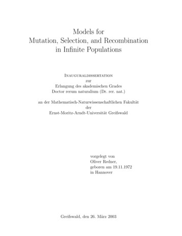
2. THE MODEL WITH DISCRETE GENOTYPEStt τtt τFigure 2: The multitype branching process. Individuals reproduce (branching lines), die(ending lines), or mutate (lines changing type) independently of each other; the various typesare indicated by different line styles. Left: The fat lines mark the clone founded by a singleindividual (bullet) at time t. Right: The fat lines mark the lines of descent defined by threeindividuals (bullets) at time t τ . After coalescence of two lines, their ancestor receives twicethe ‘weight’, as indicated by extra fat lines.The connection of this stochastic process with the deterministic model described inSectionP2.1 is twofold. Firstly, in the limit of an infinite number of individuals (i.e.,(n)(t)/n converges almostn : i ni (0) ), the sequence of random variables Ysurely to they(t) of ẏ Hy with initial condition y(0) n(0)/n [Eth86, Thm.¡ solution (n)11.2.1], Pr limn Y (t)/n y(t) 1. (The superscript (n) denotes the dependencePon the number of individuals.) The connection is now clear since p(t) : y(t)/ i yi (t)solves the mutation–selection equation (2).Secondly, taking expectations of Yi and marginalizing over all other variables, oneobtains the differential equation for the conditional expectations ¡ d ¡E Yi (t) n(0) (Bi Di )E Yi (t) n(0)dtX ¡ ¡ Mij E Yj (t) n(0) Mji E Yi (t) n(0) .(8)jClearly, the matrix H appears as the (infinitesimal) generator here, and the solution isgiven by T (t) n(0), where T (t) : exp(tH) is the corresponding¡ positive semigroup (seealso [Hof88, Ch. 11.5]). In particular, we have E Yi (t) ej Tij (t) for the expectednumber of i-individuals at time t, in a population started by a single j-individual at time0 (a ‘j-clone’). In the same way, Tij (τ ) is the expected number of descendants of type i attime t τ in a j-clone started at an arbitrary time t, cf. the left panel of Figure 2. (Notethat, due to the independence of individuals and the Markov property and homogeneityof the process on the ‘large’ state space N0 Γ , the progeny distribution depends only onthe age of the clone, and on the founder type.) Further,Pthe expected total size of aj-clone of age τ , irrespective of the descendants’ types, is i Tij (τ ).Initial conditions come into play if we consider the reproductive success of a clonerelative to the whole population. A population ofPindependent individuals, with initialcomposition p(t), has expected mean clone size i,j Tij (τ )pj (t) at time t τ (here, talways means ‘absolute’ time, whereas τ denotes a time increment). The expected sizeof a single j-clone at time t τ , relative to the expected mean clone size of the whole5

I. MUTATION–SELECTION MODELSpopulation, then iszj (τ, t) : XiTij (τ )/XTk (τ ) p (t) .(9)k, The zj express the expected relative success of a type after evolution for a time intervalτ in the sense that, if zj (τ, t) 1 ( 1), we can expect the clone to flourish more (less)than average (this does in general not mean that type j is expected to increase (decrease)in abundance relative to the initial population). Clearly, the values of the zj dependon the fitness of type j, but also on its mutation rate and the fitness of its (mutated)offspring. (If there is only mutation, but no reproduction or death, one has a Markovchain even on the ‘small’ state space Γ and zj (τ, t) 1.)We now consider lines of descent, as in the right panel of Figure 2. To this end, werandomly pick an individual alive at time t τ , and trace its ancestry back in time; thisresults in an unbranched line (in contrast to the lineage forward in time). Let Zt τ (t)denote the type found at time t t τ , ¡where we will drop the index for easier readability.We seek its probability distribution Pr Z(t) j . Since the (relative) clone size zj (τ, t)also determines the expected (relative) frequency of lines present at time t τ that containa j-type ancestor at time t, we have¡ Pr Z(t) j zj (τ, t) pj (t) : aj (τ, t) .(10)PThe aj (τ, t) define a probability distribution ( j aj (τ, t) 1), which will be of majorimportance, and may be interpreted in two ways. Forward in time, aj (τ, t) is the frequencyof j-individuals at time t, weighted by their relative number of descendants after evolutionfor some time τ . Looking backward in time, aj (τ, t) is the fraction of the (p-distributed)population at time t τ whose ancestor at time t is of type j. We shall therefore referto a(τ, t) as the ancestral distribution at the earlier time, t.Let us, at this point, expand a little further on this backward picture by explicitlyconstructing the time-reversed process. This is done in the usual way, by writing the jointdistribution of parent–offspring pairs (i.e., pairs Z(t) and Z(t τ )) in terms of forwardand backward transition probabilities. On the one hand,¡ ¡ ¡ Pr Z(t τ ) i, Z(t) j Pr Z(t τ ) i Z(t) j Pr Z(t) j(11) Pij (τ ) aj (τ, t) .¡ Here, the Pij (τ ) : Pr Z(t τ ) i Z(t) j may be obtained by rewriting theP (conditional) expectations defining the (forward) branching process as Tij (τ ) Pij (τ ) k Tkj (τ ),which givesXPij (τ ) Tij (τ )/Tkj (τ ).(12)kOn the other hand,¡ ¡ ¡ Pr Z(t τ ) i, Z(t) j Pr Z(t) j Z(t τ ) i Pr Z(t τ ) i(13) P̃ji (τ, t) pi (t τ ) ,¡ where P̃ji (τ, t) : Pr Z(t) j Z(t τ ) i is the transition probability of the time¡ 1reversed process and is obtained as P̃ji (τ, t) aj (τ, t)Pij (τ ) pi (t τ )from (11) and6

2. THE MODEL WITH DISCRETE GENOTYPES(13). With Equations (9), (10), and (12), one therefore obtains the elements of thebackward transition matrix P̃ asP̃ji (τ, t) pj (t) P 1¡Tij (τ )pi (t τ ) .k, Tk (τ ) p (t)(14)By differentiating P̃ (τ, t) with respect to τ and evaluating it at τ 0, one obtainsthe matrix Q(t) governing the correspondingbackward process in continuous time. Its ¡ ¡ 1d elements read Qji (t) dτ P̃ji (τ, t) τ 0 pj (t) Hij δij R̄(t) pi (t) δij ṗi (t)/pi (t).Using (5) this simplifies to(¡ 1pj (t)Hij pi (t)for i 6 j,¡ 1Qji (t) (15)P k6 i pk (t)Hik pi (t)for i j.Note that the backward process is, in general, state-dependent (it does not represent aMarkov chain). Note also that time reversal works in the same way if sets of types Xkinstead of single types are considered, as long as mutation and reproduction rates are thesame within classes. Furthermore, an analogous treatment is possible both for mutationcoupled to reproduction, as well as for subsequent generations.As to the asymptotic behavior of our branching process,¡ it is well-known that, forirreducible H and t , the time evolution matrix exp t(H λmax 1) becomes aprojector onto the equilibrium distribution p, with matrix elements pi zj (e.g., [Kar81,App.]).P Here, z is the Perron–Frobenius (PF) left eigenvector of H, normalized suchthat i zi pi 1. As suggested by our notation, one also haslim z(τ, t) z ,t,τ (16)which follows from (9).8 We therefore term zi the relative reproductive¡ success of type 1i.The stationary backward process is governed by the matrix Qji pj Hij δij λmax pi ,which can now be interpreted as a Markov generator. Further, the (asymptotic) ancestraldistribution, given byturns out to be the equilibriumPai zi pi , PPdistribution of the back 1ward process, since i Qji ai i pj (Hij δij λmax )pi zi pi i pj zi (Hij δij λmax ) 0.Due to ergodicity of the latter (Q is irreducible if H is), a is, at the same time, thedistribution of types along each line of descent (with probability 1).2.3The equilibrium ancestral dis

Mutation is a random change of type, which may be modeled either as taking place dur-ing reproduction or as an independent process, going on in parallel. For a review and a guide to the vast body of literature on the subject, see [Bur00, Baa00]. Certain models for coupled mutation and selection, in which genotypes are taken to be