Transcription
Graph-Theoretic Scagnostics Leland Wilkinson†Anushka Anand‡Robert Grossman§SPSS Inc.Northwestern UniversityUniversity of Illinois at ChicagoUniversity of Illinois at ChicagoA BSTRACT2We introduce Tukey and Tukey scagnostics and develop graphtheoretic methods for implementing their procedure on largedatasets.A scatterplot matrix, variously called a SPLOM or casement plotor draftman’s plot, is a (usually) symmetric matrix of pairwise scatterplots. An easy way to conceptualize a symmetric SPLOM isto think of a covariance matrix of p variables and imagine thateach off-diagonal cell consists of a scatterplot of n cases ratherthan a scalar number representing a single covariance. This displaywas first published by John Hartigan [19] and was popularized byTukey and his associates at Bell Laboratories [9]. Figure 1 shows aSPLOM of measurements on abalones using data from [27]. Off thediagonal are the pairwise scatterplots of nine variables. The variables are sex (indeterminate, male, female), shell length, shell diameter, shell height, whole weight, shucked weight, viscera weight,shell weight, and number of rings in shell.CR Categories:H.5.2 [User Interfaces]:GraphicalUser Interfaces—Visualization; I.3.6 [Computing Methodologies]:Computer Graphics—Methodology and Techniques;Keywords: visualization, statistical graphics1I NTRODUCTIONAround 20 years ago, John and Paul Tukey developed an exploratory visualization method called scagnostics. While theybriefly mentioned their invention in [42], the specifics of the methodwere never published. Paul Tukey did offer more detail at an IMAvisualization workshop a few years later, but he did not include thetalk in the workshop volume he and Andreas Buja edited [7].Scagnostics was an ingenious idea. Jerome Friedman andWerner Stuetzle, in a paper assessing John Tukey’s lifetime contributions to visualization [13], say the following:T UKEY AND T UKEY S CAGNOSTICSDraftman’s views (scatterplot matrices) lose their effectiveness when the number of variables is large. Usinga projection index similar to that in projection pursuit,the computer could find the most interesting scatterplotsto be presented to the user. John had proposals for a widevariety of scagnostic indices to judge the usefulness ofscatterplot displays. The widespread use of cognosticsand scagnostics has not yet materialized in routine dataanalysis. These approaches are perhaps among the potentially most useful of John’s yet to be explored suggestions.Scagnostics have yet to be explored by others, despite this encouragement. This may be due to the lack of published details. Inany case, this paper summarizes the Tukeys’ idea and offers a newapproach that we believe follows the spirit of their method. Ourapproach is based on recent advances in graph-theoretic summariesof high-dimensional scattered point data. We believe our methodimproves the computational efficiency and extends the scope of theoriginal idea.We will begin with a brief summary of the Tukeys’ approach,based on the first author’s recollection of the IMA workshop andsubsequent conversations with Paul Tukey. Then we will presentour graph-theoretic measures for computing scagnostic indices. Finally, we will illustrate the performance of our methods on realdata. John Hartigan, David Hoaglin, and Graham Wills provided valuablesuggestions.† e-mail: leland@spss.com‡ e-mail:aanand2@uic.edu§ e-mail:grossman@cs.uic.eduFigure 1: Scatterplot matrix of Abalone measurementsAs Friedman and Stuetzle noted, scatterplot matrices become unwieldy when there are many variables. First of all, the visual resolution of the display is limited when there are many cells. Thisdefect can be ameliorated by pan and zoom controls. More critical,however, is the multiplicity problem in visual exploration. Lookingfor patterns in p(p 1)/2 scatterplots is impractical when there aremany variables. This problem prompted the Tukeys’ approach.The Tukeys reduced an O(p2 ) visual task to an O(k2 ) visualtask, where k is a small number of measures of the distributionof a 2D scatter of points. These measures included the area ofthe peeled convex hull [40] of the 2D point scatters, the perimeter length of this hull, the area of closed 2D kernel density isolevelcontours [35], [33], the perimiter length of these contours, the convexity of these contours, a modality measure of the 2D kernel densities, a nonlinearity measure based on principal curves [21] fittedto the 2D scatterplots, and several others. By using these measures,
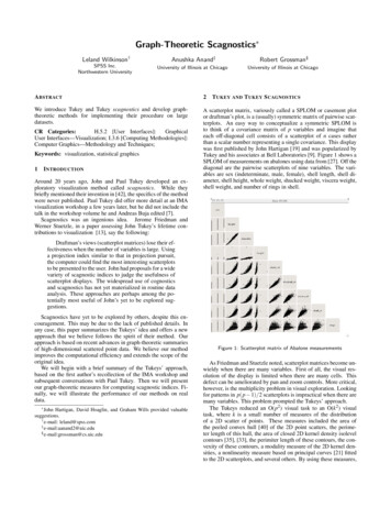
the Tukeys aimed to detect anomalies in density, shape, trend, andother features in the 2D point scatters.After calculating these measures, the Tukeys constructed a scatterplot matrix of the measures themselves. This step amounted toa level of indirection, like a pointer, in which each point in thescagnostic SPLOM represented a scatterplot cell in the originaldata SPLOM. With brushing and linking tools, unusual scatterplotscould be identified from outliers in the scagnostic SPLOM.In his IMA talk, Paul Tukey mentioned an additional step wemight take. The scagnostic SPLOM can be thought of as a visualization of a set of pointers. We can therefore construct a set ofpointers to pointers. In doing so, we can locate unusual clusters ofmeasures that characterize unusual clusters of raw scatterplots.3G RAPH -T HEORETIC S CAGNOSTICSThere are two aspects of the Tukeys’ approach that can be improved. First, some of the Tukeys’ measures, particularly thosebased on kernels, presume an underlying continuous empirical ortheoretical probability function. This is appropriate for scatterssampled from continuous distributions, but it can be a problem forother types of data. Second, the computational complexity of someof the Tukey measures is O(n3 ). Since n was expected to be smallfor most statistical applications of this method, such complexitywas not expected to be a problem.We can ameliorate both these problems by using graph-theoreticmeasures. Indeed, the Tukeys used a few themselves. First, thegraph-theoretic measures we will use do not presume a connectedplane of support. They can be metric over discrete spaces. Second,the measures we will use are O(n log(n)) in the number of pointsbecause they are based on subsets of the Delaunay triangulation.Third, we employ adaptive hexagon binning [8] before computingour graphs to further reduce the dependence on n.There is a price for switching to graph-theoretic measures, however. They are highly influenced by outliers and singletons. Whenever practical, the Tukeys used robust statistical estimators to downweight the influence of outliers. We will follow their example byworking with nonparametric and robust measures. Further, we willremove outlying points in the minimum spanning tree before computing our graphs and the measures based on them.We next introduce some notation for the projections underlyingthe scagnostics idea.3.1Remark 1. Given a data set X R p containing n points, we areinterested in the scatterplot matrix of X and the scatterplot matrixof τ(X).Remark 2. Note that the same definition works for k measuresdefined on projections in higher dimensional spaces. For example,we can work with projections in three space, with X[i, j,k] denotingthe set (πi π j πk )(X) R3 .We next introduce and define the graphs we will use as bases forour measures and then we discuss the measures themselves.3.2Geometric GraphsA graph G {V, E} is a collection of a set of vertices V and aset of edges E. An edge e(v, w), with e E and v, w V , is anunordered pair of vertices. A geometric graph G? [ f (V ), g(E), S]is an embedding of a graph in a metric space S that maps verticesto points and edges to line segments connecting pairs of points.We will omit the asterisk in the rest of this paper and assume allour graphs are geometric. We will also restrict our candidates togeometric graphs that are: undirected (edges consist of unordered pairs) simple (no edge pairs a vertex with itself) planar (there is an embedding in R2 with no crossed edges) straight (embedded eges are straight line segments) finite ( V and E are finite sets)See [12] for alternatives.Figure 2 shows instances of the geometric graphs on which wewill compute our measures. The points are taken from one of thecells in the abalone SPLOM. In this section, we define the geometric graphs that are the bases for our measures.Scagnostic Projections Let πi denote the projectionR p R,Figure 2: Graphs used as bases for computing scagnostics measuresx xion the ith coordinate. Let πi π j denote the projectionp2R R ,3.2.1x (xi , x j ). Given a set X R p , let X[i, j] denote the set (πi π j )(X) R2 .We will be interested in the p(p 1)/2 different data sets X[i, j]formed by varying i, j 1, . . . , p where i j.To define the scagnostics transform, we first need to fix k measures c1 , . . ., ck defined on sets X in R2 . For example, c1 can be ameasure of the central location of the points, c2 can be a measureof the dispersion of the points, and so on.Given a data set X containing n points in R p , the scagnosticstransform τ(X) is the data set of p(p 1)/2 points in Rk containingthe following points:(c1 (X[i, j] ), . . . , ck (X[i, j] )) Rk ,i, j 1, . . . , p,i j.Convex HullA polygon is a closed planar region with n vertices and n 1 faces.The boundary of a polygon can be represented by a geometric graphwhose vertices are the polygon vertices and whose edges are thepolygon faces. A hull of a set of points X in R2 is a collection ofone or more boundaries of polygons that have a subset of the pointsin X for their vertices and that collectively contain all the points inX. This definition includes entities that range from the boundaryof a single polygon to a collection of boundaries of polygons eachconsisting of a single point.We now define the convex hull. A set of points X in R2 is convexif it contains all the straight line segments connecting any pair of itspoints. The convex hull of X is the boundary of the intersection ofall convex sets containing X. This definition implies that the convexhull is the boundary of a convex polygon and that its vertices consistof points in X.
There are several algorithms for computing the convex hull [36].Since the convex hull consists of the outer edges of the Delaunaytriangulation, we can use an algorithm for the Voronoi/Delaunayproblem and then pick the outer edges. Its computation thus canbe O(n log(n)). We will use the convex hull, together with othergraphs, to construct measures of convexity.3.2.2Nonconvex HullA nonconvex hull is a hull that is not the convex hull. This class includes simple shapes like a star convex or monotone convex hull [3],but it also includes some space-filling, snaky objects and some thathave disjoint parts. In short, we are interested in a general class ofnonconvex shapes.There have been several geometric graphs proposed for representing the “shape” of a set of points X on the plane. Most of theseare proximity graphs [23]. A proximity graph (or neighborhoodgraph) is a geometric graph whose edges are determined by an indicator function based on distances between a given set of points ina metric space. To define this indicator function, we use an opendisk D. We say D touches a point if that point is on the boundaryof D. We say D contains a point if that point is in D. We call thesmallest open disk touching two points D2 ; the radius of this disk ishalf the distance between the two points and the center of this diskis halfway between the two points. We call an open disk of fixedradius D(r). We call an open disk of fixed radius and centered on apoint, D(p, r).We considered several candidates for a shape-revealing proximity graph on a set of planar points. Some of them are subsets of theDelaunay triangulation: In a Delaunay graph, an edge exists between any pair ofpoints that can be touched by an open disk D containing nopoints. The external edges of the Delaunay triangulation arethe convex hull. This means that the external edges of the Delaunay graph cannot be used to represent non-convex hulls. A beta skeleton graph [25] is a close relative of the relativeneighborhood graph. It uses a lune whose size is determinedby a parameter β .We have chosen the alpha hull for deriving our measures ofshape. An alpha hull is a nonconvex hull derived from the boundary of an alpha shape graph. There are several reasons behind ourchoice. First, the alpha shape is relatively efficient to compute because it is a subset of the Delaunay triangulation with a simple inclusion criterion. Second, it is an erosion method. This aspect ofthe algorithm suits statistical data because we are interested in reducing the influence of outlying points on a shape.A problem with using the alpha hull for a shape detector ischoosing the value of the α parameter (the radius of the disk that isused to delete edges in the Delaunay triangulation). We choose α tobe the value of the ω parameter (discussed below). The ω parameter is the cutoff value for identifying outlying edges in the minimumspanning tree. We choose this value because we wish to erase edgesin the Delaunay triangulation that are longer than outlying edges inthe original MST.3.2.3Minimum Spanning TreeA tree is an acyclic, connected, simple graph. A spanning tree is anundirected graph whose edges are structured as a tree. A minimumspanning tree (MST) is a spanning tree whose total length (sumof edge weights) is least of all spanning trees on a given set ofpoints [24]. The edge weights of a geometric MST are computedfrom distances between its vertices.The MST is a subgraph of the Delaunay triangulation. Thereare several efficient algorithms for computing an MST for a set ofpoints in the plane [28], [31].3.3Measures In a Gabriel graph [15], an edge exists between any pair ofpoints that have a D2 containing no points.We are interested in assessing five aspects of scattered points: outliers, shape, trend, density, and coherence. Our measures are derived from several features of geometric graphs: In a relative neighborhood graph [39], an edge exists betweenany pair of points p and q for which r is the distance betweenp and q and the intersection of D(p, r) and D(q, r) contains nopoints. This intersection region is called a lune. The length of an edge, length(e), is the Euclidean distancebetween its vertices. In an alpha shape graph [10], an edge exists between any pairof points that can be touched by an open disk D(α) containingno points. The length of a graph, length(G), is the sum of the lengths ofits edges. A path is a list of vertices such that all pairs of adjacent vertices in the list are edges.Others are not subsets of the Delaunay: In a distance graph, an edge exists between any pair of pointsthat both lie in a D(r). The radius r defines the size of theneighborhood. This graph is not always planar and is therefore not a subset of the Delaunay. In a k-nearest neighbor graph (KNN), a directed edge existsbetween a point p and a point q if d(p, q) is among the k smallest distances in the set {d(p, j) 1 j n, j 6 p}. Mostapplications restrict KNN to a simple graph by removing selfloops and edge weights. If k 1, this graph is a subset of theMST. If k 1, this graph is not always planar. In a sphere of influence graph [5], an edge exists betweena point p and a point q if d(p, q) dnn (p) dnn (q), wherednn (.) is the nearest-neighbor distance for a point. A path is closed if its first and last vertex are the same. A closed path is the boundary of a polygon. The perimeter of a polygon, perimeter(P), is the length of itsboundary. The area of a polygon, area(P) is the area of its interior. The diameter of a graph, diameter(G), is the longest shortestpath in G.All our measures are defined to be in the closed unit interval. Tocompute them, we assume our variables are scaled to the closedunit interval as well.
3.3.1 StringyOutliersTukey [40] introduced the use of the peeled convex hull as a measure of the depth of a level set imposed on scattered points. Forpoints on the 1D line, this amounts to successive symmetric trimming of extreme observations. Tukey’s idea can be used as an outlier identification procedure. We compute the convex hull, deletepoints on the hull, compute the convex hull on the remaining points,and continue until (one hopes) the contours of successive hulls donot substantially differ.We have taken a different approach. Because we do not assumethat our point sets are convex (that is, comparably dense in all subregions of the convex hull), we cannot expect outliers will be on theedges of a convex hull. They may be located in interior, relativelyempty regions. Consequently, we have chosen to peel the MST instead of the hull. We consider an outlier to be a vertex with degree1 and associated edge weight greater than ω.There are theoretical results on the distribution of the largestedge for an MST on normally distributed data [30], but we decidedto work with a nonparametric criterion for simplicity. FollowingTukey [41], we chooseω q75 1.5(q75 q25 )where q75 is the 75th percentile of the MST edge lengths and theexpression in the parentheses is the interquartile range of the edgelengths. OutlyingA stringy shape is a skinny shape with no branches. Thestringy measure is based on the π index, which is the ratioof width to length of a network. If the longest shortest paththrough a minimum spanning tree is almost as long as the sumof all the edges in the tree itself, then the tree is path-like orstringy.cstringy diameter(T )/length(T ) StraightThe spanning ratio or dilation of a geometric graph is themaximum ratio (over all pairs of vertices) of the shortest path(geodesic) between two vertices and the Euclidean distancebetween same vertices. Because it jumps to nearest neighbors,the MST has a dilation of O(n) [11]. For a perfectly linear geometric graph (all points in general position), the MST has aspanning ratio of 1.We invert this ratio so that a straight graph has a value of 1and other graphs have a smaller value. We modify this ratiofurther, however. Our ratio is the Euclidean distance betweenthe points at the ends of the longest shortest path of the MSTdivided by the longest shortest path itself (the diameter of theMST). Even if the Pearson correlation is zero, our straightnessindex will be large for a set of points lying near a straight line.We will leave it to our monotonicity index to pick up scattersthat are straight and highly correlated. Thus, our measure isThis is a measure of the proportion of the total edge length dueto extremely long edges connected to points of single degree.coutlying length(Toutliers )/length(T )3.3.2cstraight dist(t j ,tk )/diameter(T )where t j and tk are the vertices in T on which the diameter isdefined.3.3.3ShapeThe shape of a set of scattered points is our next consideration. Weare interested in both topological and geometric aspects of shape.We want to know, for example, whether a set of scattered points onthe plane appears to be connected, convex, inflated, and so forth. Ofcourse, scattered points are by definition not these things, so we aregoing to need additional machinery (based on our graphs that we fitto these points) to allow us to make such inferences. The measuresthat we propose will be based on these graphs.In the formulas below, we use H for the convex hull, A for thealpha hull, and T for the minimum spanning tree. In our shapecalculations, we ignore outliers. ConvexThis is the ratio of the area of the alpha hull and the area ofthe convex hull. This ratio will be 1 if the nonconvex hull andthe convex hull have identical areas.cconvex area(A)/area(H) SkinnyThe following index helps reveal whether a given scatter ismonotonic. MonotonicIf a set of scattered points is functional on x (plus error), amonotonicity coefficient should assess whether that functionis monotonic. We have chosen the squared Spearman correlation coefficient, which is a Pearson correlation on the ranksof x and y (corrected for ties). We square the coefficient to accentuate the large values and remove the distinction betweennegative and positive coefficients. We assume investigatorsare most interested in strong relationships, whether negativeor positive.cmonotonic r2 spearmanThis is our only coefficient not based on a subset of the Delaunay graph. Because it requires a sort, its computation isO(n log(n)).3.3.4The ratio of perimeter to area of a polygon measures, roughly,how skinny it is. We use a corrected and normalized ratio sothat a circle yields a value of 0, a square yields 0.12 and askinny polygon yields a value near one.pcskinny 1 4πarea(A)/perimeter(A)TrendDensityThe following indices detect different distributions of points. SkewedThe distribution of edge lengths of a minimum spanningtree gives us information about the relative density of pointsin a scattered configuration. Some have used the sample
mesh on x. Nor will it detect large negative autocorrelationstructures, for similar reasons. Instead, we expect this measure to have large values when a series is relatively smooth.Furthermore, our measure does not assume a path is singlevalued on x.mean, variance, and skewness statistics to summarize thisedge length distribution, e.g., [1]. However, theoretical results [37], [30] show that the MST edge-length distributionfor many types of point scatters can be approximated by anextreme value distribution with fewer parameters. Other theoretical results [17] suggest that the mean MST edge lengthfor a geometric graph on the unit square depends more onthe number of points than on the distribution of points. OurMonte Carlo simulations using the distributions in Figure 3found little variation in mean MST edge length for fixed n.By contrast, the skewness of the histograms of the MST edgelength distributions for these points varied considerably. Consequently, we use a simple measure of skewness based on aratio of quantiles of the edge lengths. StriatedThe bottom scatterplot in Figure 3 shows points on parallellines. We could recognize this pattern with a Hough transform [22]. Other configurations of points that represent vector flows or striated textures might not follow linear paths,however. We are interested in a more general measure. Recognizing that almost all of the adjacent edges in the MST onthese points are collinear. Graham Wills (personal communication) proposed the following measure, which sums anglesover all adjacent edges. Let V (2) V be the set of all verticesof degree 2 in V . Thencskew (q90 q50 )/(q90 q10 )This statistic is relatively robust to outliers. Clumpycstriate (T ) An extremely skewed distribution of MST edge lengths doesnot necessarily indicate clustering of points. For this, we turnto another measure based on the MST: the Hartigan and Mohanty RUNT statistic [20]. This statistic is most easily understood in terms of the single-linkage hierarchical clusteringtree called a dendrogram. The runt size of a dendrogram nodeis the smaller of the number of leaves of each of the two subtrees joined at that node. Since there is an isomorphism between a single-linkage dendrogram and the MST [18], we canassociate a runt size (r j ) with each edge (e j ) in the MST, asdescribed by Stuetzle [38]. The runt graph (R j ) correspondingto each edge is the smaller of the two subsets of edges that arestill connected to each of the two vertices in e j after deletingedges in the MST with lengths less than length(e j ).Our runt-based measure emphasizes clusters with small intracluster distances relative to the length of their connecting edgeand ignores runt clusters with relatively small runt size. cclumpy (T ) max 1 max [length(ek )] /length(e j )jBinningWe use hexagon binning [8] to improve performance. We beginwith a 40 by 40 hexagon grid for each scatterplot. If there are morethan 250 nonempty cells, we reduce the bin size by half and rebin.We continue this process until there are no more than 250 nonemptycells.We examined by Monte Carlo simulation the effect of binningon our measures. Because we designed the measures to minimizethis effect, the only one that showed a substantial trend with binsize was the stringy index. Not surprisingly, substantially larger binsizes produce a higher index. Small edges are lost in larger bins,so the denominator of the index decreases with increase in bin size.We tried several adjustments to the index, including estimating thewithin-bin size of edges and adding this estimate to the denominator. All of the adjustments we tried substantially reduced thesensitivity of the measure, so we decided to leave the stringy indexunadjusted.kwhere j indexes edges in the MST and k indexes edges in eachrunt set derived from an edge indexed by j.3.3.53.41 cos θe(v,a)e(v,b) V (2) v V (2)CoherenceWe define coherence in a set of points as the presence of relatively smooth paths in the minimum spanning tree. Smoothalgebraic functions, time series, and curves (e.g., spirals) fitthis definition. So do points arranged in flows or vector fields.There are numerous diagnostic measures for time series. Mostof these involve conditioning on a model and examining residuals for lack of independence. For stochastic series, diagnostics usually assume stationarity in order for the tests to bevalid. Stationarity implies that the mean, variance and autocorrelation structure of a process are defined and do notchange over time. Verifying this can be problematic and timeconsuming.We have chosen an alternative approach by devising a robustmeasure of coherence. This measure is not intended to be atime series detector. Not every time series is smooth. Forexample, moving average processes such as MA(1) may oscilllate at frequencies that are higher than the resolution of the4P ERFORMANCEFigure 3 shows the results of our graph-theoretic measures appledto 11 different scatter patterns. We notice that the red or orangerectangles align with patterns the respective measures are designedto flag.We can get a graphical idea of the sensitivity and specificityof the measures by examining the first two principal componentsof these measures applied to these patterns. Figure 4 shows a biplot [16] of the measures and patterns. We find that the measuresfill the space and are near the patterns they target. The clumpy measure has a short vector in the plot because it loads heavily on a thirdcomponent. The scree (plot of eigenvalues against factor indices) issmoothly descending with no clear elbow, so the dimensionality ofthese measures on the selected point sets is not low.4.1TimeBecause we use binning and efficient triangulation, computationtime is roughly O(np2 ). On a Macintosh G4 PowerBook runningJava 1.4.2, computing the measures on 100,000 random cases distributed uniformly on 10 variables requires approximately 10 seconds. Computing the measures on 100,000 cases and 25 variablesrequires approximately 75 seconds. Large, uniformly distributed
Figure 4: Biplot of measures and scattersFigure 3: Scaled graph-theoretic measures (blue low, red high) foreleven scatter patternspoint sets tend to increase computation time because of the needfor rebinning. Datasets with compact, nonuniform distributions areconsiderably faster to compute.5E XAMPLESFigure 5 shows a scagnostics SPLOM for the Abalone dataset. Wehave highlighted a point in the SPLOM that represents one unusualscatterplot. The linked plot is shown in the upper right of the figure.From what we see in the SPLOM, we can characterize this scatterplot as relatively high in outliers, skewed in edge lengths, clumpy,nonconvex, striated, and stringy.Figure 6 shows a scagnostics SPLOM of 17 variables from adataset based on statistics for selected countries compiled by theWorld Health Organization and the United Nations [43]. We havehighlighted a point in the graph-theoretic SPLOM to give an example of the type of anomalies that scagnostics can uncover. Thered point is clearly an outlier in most of the panels. The scatterplotcorresponding to this point is shown in the upper right of the figure. We were surprised to find that we had included two versionsof a categorical variable measuring the type of government – onerecoded to have fewer categories. Because these two artifactuallyrelated variables are not perfectly correlated, they would have nothave induced a singularity in a statistical analysis and might havebeen undetected in a thoughtless automated data mining.Figure 7 shows a scagnostics SPLOM of 62 variables from amicroarray dataset [2]. The SPLOM shows the high degree ofhomogeneity in the 2D marginal distributions of the 62 cell linesin the array. The linked scatterplot shows a typical 2D distribution, evidently not bivariate normal. The authors identified clusters of non-cancerous and cancerous cells in these data. We mustremember that lack of evidence for clusters in the 2D scatters isnot evidence for lack of clusters in higher dimensions. Instead, thescagnostic SPLOM lends some support to the authors’ findings bydownweighting the possibility that clusters might be due to measurement artifacts (e.g., mixing discrete and continuous variablesin the analysis). This application illlustrates the appropriate focusof scagnostics as a preliminary screening method.Figure 8 shows a SPLOM of weather data. The data comprisehourly meteorological measurements over a year at the GreenlandHumboldt automatic weather station operated by NASA and NSF.These measurements are part of the Greenland Climate Network(GC-Net) sponsored by these federal agencies. We have sortedthe variables in the SPLOM using the size of the loadings on thefirst principal component of the scagnostic measures. The sortingclearly segregates the discrete and continuous variables and clusterssimilar marginal 2D distributions.6C ONCLUSIONAs we have seen, scagnostics offers the possibility of detectingano
Graph-Theoretic Scagnostics Leland Wilkinson† SPSS Inc. Northwestern University Anushka Anand‡ University of Illinois at Chicago Robert Grossman§ University of Illinois at Chicago