Transcription
Visualizing DataCarlos HurtadoDepartment of EconomicsUniversity of Illinois at Urbana-Champaignhrtdmrt2@illinois.eduOct 3rd, 2017C. Hurtado (UIUC - Economics)Numerical Methods
On the Agenda12D Figures in Python2Matplotlib vs. Pylab3Saving a Figure4Detailed Graphs5Two ore more graphs in one figure6Histograms7Colormaps and Contour83D PlotsC. Hurtado (UIUC - Economics)Numerical Methods
2D Figures in PythonOn the Agenda12D Figures in Python2Matplotlib vs. Pylab3Saving a Figure4Detailed Graphs5Two ore more graphs in one figure6Histograms7Colormaps and Contour83D PlotsC. Hurtado (UIUC - Economics)Numerical Methods
2D Figures in Python2D Figures in PythonI The purpose of scientific computation is insight, not only numbersI To understand the meaning of the numbers we compute, we oftenneed post-processing, statistical analysis and graphical visualization ofour data.I The Python library Matplotlib is a python 2D plotting library whichproduces quality figures.I You can generate histograms, bar charts, scatter plots, etc.I Matplotlib as an object oriented plotting library.I Pylab is an interface to the same set of functionsC. Hurtado (UIUC - Economics)Numerical Methods1 / 15
Matplotlib vs. PylabOn the Agenda12D Figures in Python2Matplotlib vs. Pylab3Saving a Figure4Detailed Graphs5Two ore more graphs in one figure6Histograms7Colormaps and Contour83D PlotsC. Hurtado (UIUC - Economics)Numerical Methods
Matplotlib vs. PylabMatplotlib vs. PylabI Pylab is slightly more convenient to use for easy plotsI Matplotlib gives far more detailed control over how plots are created.I Let us compute our first example123456 import numpy as npimport matplotlib . pyplot as pltx np . arange ( -3.14 ,3.14 ,0.01)y np . sin ( x )plt . plot (x , y )plt . show ()C. Hurtado (UIUC - Economics)Numerical Methods2 / 15
Matplotlib vs. PylabMatplotlib vs. PylabI Pylab is slightly more convenient to use for easy plotsI Matplotlib gives far more detailed control over how plots are created.I Let us compute our first example123456 import numpy as npimport matplotlib . pyplot as pltx np . arange ( -3.14 ,3.14 ,0.01)y np . sin ( x )plt . plot (x , y )plt . show ()C. Hurtado (UIUC - Economics)Numerical Methods2 / 15
Matplotlib vs. PylabMatplotlib vs. PylabI We could also have written the previous example as follows:123456 import pylabimport numpy as npx np . arange ( -3.14 ,3.14 ,0.01)y np . sin ( x )pylab . plot (x , y )pylab . show ()C. Hurtado (UIUC - Economics)Numerical Methods3 / 15
Matplotlib vs. PylabMatplotlib vs. PylabI We could also have written the previous example as follows:123456 import pylabimport numpy as npx np . arange ( -3.14 ,3.14 ,0.01)y np . sin ( x )pylab . plot (x , y )pylab . show ()C. Hurtado (UIUC - Economics)Numerical Methods3 / 15
Saving a FigureOn the Agenda12D Figures in Python2Matplotlib vs. Pylab3Saving a Figure4Detailed Graphs5Two ore more graphs in one figure6Histograms7Colormaps and Contour83D PlotsC. Hurtado (UIUC - Economics)Numerical Methods
Saving a FigureSaving a FigureI Once you have created the figure you can save it directly from yourPython code.I To do that, it is ideal to know your current working directoryI The Module os provides a way of using operating system dependentfunctions.I The following code will give you the path to your current workingdirectory1234 import os cwd os . getcwd () print cwd/ home / Carlos / Desktop /I To set the directory where you want to save your work, you can usethe function chdir in the module os1 od . chdir ( " / home / Carlos / Desktop / L4 / " )C. Hurtado (UIUC - Economics)Numerical Methods4 / 15
Saving a FigureSaving a FigureI To save the figures using the object oriented Matplotlib, we need tocreate an object to save the figure12345 od . chdir ( " / home / Carlos / Desktop / L4 / " )fig plt . figure ()plt . plot (x , y )plt . show ()fig . savefig ( " fig1 . png " )I The object fig on the previous code will contain the plotI The following code will have the same effect:1 fig plt . figure ()2 plt . plot (x , y )3 fig . savefig ( " fig1 . png " )I The important part is to generate the object fig before doing usingthe module pltC. Hurtado (UIUC - Economics)Numerical Methods5 / 15
Saving a FigureSaving a FigureI We don’t need to create an object to save using the module pylabI However, we cannot use the ’show’ function before saving using themodule pylab1 pylab . plot (x , y )2 pylab . savefig ( ’ fig2 . png ’)I You can also save files in different formats by changing the extensionof the file1 pylab . plot (x , y )2 pylab . savefig ( ’ fig2 . pdf ’)I The pdf format is a vector file, that means that one can ’zoom in’ theimage without loosing quality.I File formats such as png (and jpg, gif, tif, bmp) save the image inform of a bitmap (i.e. a matrix of colour values)C. Hurtado (UIUC - Economics)Numerical Methods6 / 15
Detailed GraphsOn the Agenda12D Figures in Python2Matplotlib vs. Pylab3Saving a Figure4Detailed Graphs5Two ore more graphs in one figure6Histograms7Colormaps and Contour83D PlotsC. Hurtado (UIUC - Economics)Numerical Methods
Detailed GraphsDetailed GraphsI Matplotlib and Pylab allows us to fine tune our plots in great detail.1234567891011121314 import pylabimport numpy as npx np . arange ( -3.14 ,3.14 ,0.01)y1 np . sin ( x )y2 np . cos ( x )pylab . figure ( figsize (5 ,5) )pylab . plot (x , y1 , label ’ sin ( x ) ’)pylab . plot (x , y2 , label ’ cos ( x ) ’)pylab . legend ()pylab . grid ()pylab . xlabel ( ’x ’)pylab . ylabel ( ’y ’)pylab . title ( ’ My nice graph ’)pylab . show ()C. Hurtado (UIUC - Economics)Numerical Methods7 / 15
Detailed GraphsMy nice graph1.0sin(x)cos(x)y0.50.00.51.04C. Hurtado (UIUC - Economics)3210x1Numerical Methods2347 / 15
Detailed GraphsDetailed GraphsI Use the help for more information on how to use the plot function1 help ( " pylab . plot " )I By calling the plot command repeatedly, more than one curve can bedrawn in the same graph.12345 t np . arange (0 ,2* np . pi ,0.01)pylab . plot (t , np . sin ( t ) , label " sin ( t ) " )pylab . plot (t , np . cos ( t ) , ’g - - ’ , label " cos ( t ) " )pylab . legend ()pylab . savefig ( ’ fig4 . png ’)C. Hurtado (UIUC - Economics)Numerical Methods8 / 15
Detailed GraphsDetailed GraphsI Use the help for more information on how to use the plot function1 help ( " pylab . plot " )I By calling the plot command repeatedly, more than one curve can bedrawn in the same graph.12345 t np . arange (0 ,2* np . pi ,0.01)pylab . plot (t , np . sin ( t ) , label " sin ( t ) " )pylab . plot (t , np . cos ( t ) , ’g - - ’ , label " cos ( t ) " )pylab . legend ()pylab . savefig ( ’ fig4 . png ’)C. Hurtado (UIUC - Economics)Numerical Methods8 / 15
Detailed GraphsDetailed GraphsI We can plot more than one curve using the matplotlib.pyplot module1234567 fig , ax plt . subplots ()t np . arange (0 ,2* np . pi ,0.01)ax . plot (t , np . sin ( t ) , label " sin ( t ) " )ax . plot (t , np . cos ( t ) ,"g - - " , label " cos ( t ) " )ax . legend ( loc 0)plt . show ()fig . savefig ( " fig5 . png " )C. Hurtado (UIUC - Economics)Numerical Methods9 / 15
Two ore more graphs in one figureOn the Agenda12D Figures in Python2Matplotlib vs. Pylab3Saving a Figure4Detailed Graphs5Two ore more graphs in one figure6Histograms7Colormaps and Contour83D PlotsC. Hurtado (UIUC - Economics)Numerical Methods
Two ore more graphs in one figureTwo ore more graphs in one figureI We can arrange several graphs within one figure windowI The general syntax is:1 subplot ( numRows , numCols , plotNum )I For example, to arrange 4 graphs in a 2-by-2 matrix, and to select thefirst graph for the next plot command, one can use1 subplot (2 ,2 ,1)C. Hurtado (UIUC - Economics)Numerical Methods10 / 15
Two ore more graphs in one figureTwo ore more graphs in one figureI Example:12345678910111213 import numpy as npimport pylabt np . arange (0 ,2* np . pi ,0.01)pylab . subplot (2 ,1 ,1)pylab . plot (t , np . sin ( t ) )pylab . xlabel ( ’t ’)pylab . ylabel ( ’ sin ( t ) ’)pylab . subplot (2 ,1 ,2)pylab . plot (t , np . cos ( t ) , ’g - - ’)pylab . xlabel ( ’t ’)pylab . ylabel ( ’ cos ( t ) ’)pylab . savefig ( ’ fig6 . png ’)pylab . show ()C. Hurtado (UIUC - Economics)Numerical Methods11 / 15
Two ore more graphs in one figureTwo ore more graphs in one t)0.50.00.51.00C. Hurtado (UIUC - Economics)tNumerical Methods11 / 15
Two ore more graphs in one figureTwo ore more graphs in one figureI Example2:1234567891011121314151617181920 i m p o r t numpy a s npimport m a t p l o t l i b . p y p l o t as p l tx np . l i n s p a c e ( 0 . 7 5 , 1 , 1 0 0 )n np . a r r a y ( [ 0 , 1 , 2 , 3 , 4 , 5 ] )f i g , a x e s p l t . s u b p l o t s ( 2 , 2 , f i g s i z e ( 6 , 6 ) )a x e s [ 0 , 0 ] . s c a t t e r ( x , x 0 . 2 5 np . random . r a n d n ( l e n ( x ) ) )axes [ 0 , 0 ] . s e t t i t l e ( ” s c a t t e r ” )a x e s [ 0 , 0 ] . s e t x l a b e l ( ” x1 ” )a x e s [ 0 , 1 ] . s t e p ( n , n 2 , lw 2)axes [ 0 , 1 ] . s e t t i t l e ( ” step ” )axes [ 0 , 1 ] . s e t x l a b e l ( ”n” )a x e s [ 1 , 0 ] . b a r ( n , n 2 , a l i g n ” c e n t e r ” , w i d t h 0 . 8 , a l p h a 0 . 5 , c o l o r ” o r a n g e ” )axes [ 1 , 0 ] . s e t t i t l e ( ” bar ” )axes [ 1 , 0 ] . s e t x l a b e l ( ” bin ” )a x e s [ 1 , 1 ] . f i l l b e t w e e n ( x , x 2 , x , a l p h a 0 . 5 , c o l o r ” g r e e n ” )axes [ 1 , 1 ] . s e t t i t l e ( ” f i l l b e t w e e n ” )a x e s [ 1 , 1 ] . s e t x l a b e l ( ” x2 ” )axes [ 1 , 1 ] . s e t x l i m (0 ,1)axes [ 1 , 1 ] . s e t y l i m (0 ,1)f i g . s a v e f i g ( ’ f i g 7 . png ’ )C. Hurtado (UIUC - Economics)Numerical Methods12 / 15
Two ore more graphs in one figureTwo ore more graphs in one 0.50.0x10.51.01.5bar2500.8150.6100.450.21C. Hurtado (UIUC - Economics)012bin134560.00.02n3450.81.0fill between1.020000.2Numerical Methods0.4x20.612 / 15
HistogramsOn the Agenda12D Figures in Python2Matplotlib vs. Pylab3Saving a Figure4Detailed Graphs5Two ore more graphs in one figure6Histograms7Colormaps and Contour83D PlotsC. Hurtado (UIUC - Economics)Numerical Methods
HistogramsHistogramsI Example:123456789101112131415 i m p o r t numpy a s npfrom s c i p y . s t a t s i m p o r t normimport m a t p l o t l i b . p y p l o t as p l t(mu , s i g m a ) ( 1 0 0 , 1 5 )x mu s i g m a np . random . r a n d n ( 1 0 0 0 0 )f i g plt . figure ()n , b i n s , p a t c h e s p l t . h i s t ( x , 5 0 , normed 1 , f a c e c o l o r ’ g r e e n ’ , a l p h a 0.75)plt . xlabel ( ’x ’)plt . ylabel ( ’ Probability ’)p l t . t i t l e ( ’ H i s t o g r a m : mu 100 , s i g m a 15 ’ )p l t . a x i s ( [ 4 0 , 160 , 0 , 0 . 0 3 ] )p l t . g r i d ( True )y norm . p d f ( b i n s , mu , s i g m a )p l t . p l o t ( b i n s , y , ’ r ’ , l i n e w i d t h 1)p l t . show ( )C. Hurtado (UIUC - Economics)Numerical Methods13 / 15
HistogramsHistogramsHistogram: mu 100, sigma C. Hurtado (UIUC - Economics)6080100xNumerical Methods12014016013 / 15
Colormaps and ContourOn the Agenda12D Figures in Python2Matplotlib vs. Pylab3Saving a Figure4Detailed Graphs5Two ore more graphs in one figure6Histograms7Colormaps and Contour83D PlotsC. Hurtado (UIUC - Economics)Numerical Methods
Colormaps and ContourColormaps and ContourI Example:123456 .789101112131415161718 i m p o r t numpy a s npimport m a t p l o t l i balpha 0.7p h i e x t np . p id e f f l u x q u b i t p o t e n t i a l ( phi m , p h i p ) :r e t u r n 2 a l p h a 2 np . c o s ( p h i p ) np . c o s ( p h i m ) a l p h a np . c o s (p h i e x t 2 p h i p )p h i m np . l i n s p a c e ( 0 , 2 np . p i , 1 0 0 )p h i p np . l i n s p a c e ( 0 , 2 np . p i , 1 0 0 )X , Y np . m e s h g r i d ( p h i p , p h i m )Z f l u x q u b i t p o t e n t i a l (X , Y) . Tf i g , ax p l t . s u b p l o t s ( )p ax . p c o l o r (X , Y , Z , cmap m a t p l o t l i b . cm . RdBu , vmin Z . min ( ) , vmax Z . max ( ) )ax . s e t x l i m ( 0 , 2 np . p i )ax . s e t y l i m ( 0 , 2 np . p i )f i g . c o l o r b a r ( p , ax ax )f i g . show ( )f i g , ax p l t . s u b p l o t s ( )ax . c o n t o u r ( Z , cmap m a t p l o t l i b . cm . RdBu , vmin Z . min ( ) , vmax Z . max ( ) , e x t e n t [0 ,2 np . p i , 0 , 2 np . p i ] )C. Hurtado (UIUC - Economics)Numerical Methods14 / 15
Colormaps and ContourColormaps and Contour65.054.544.03.533.022.512.001.50C. Hurtado (UIUC - Economics)1234Numerical Methods5614 / 15
Colormaps and ContourColormaps and Contour65432100C. Hurtado (UIUC - Economics)123Numerical Methods45614 / 15
3D PlotsOn the Agenda12D Figures in Python2Matplotlib vs. Pylab3Saving a Figure4Detailed Graphs5Two ore more graphs in one figure6Histograms7Colormaps and Contour83D PlotsC. Hurtado (UIUC - Economics)Numerical Methods
3D Plots3D PlotsI Example:12345678910 i m p o r t m a t p l o t l i b . p y p l o t a s p l t from m p l t o o l k i t s . m p l o t 3 d . a x e s 3 d i m p o r t Axes3D f i g p l t . f i g u r e ( f i g s i z e ( 1 4 , 6 ) ) ax f i g . a d d s u b p l o t ( 1 , 2 , 1 , p r o j e c t i o n ’ 3d ’ ) ax . p l o t s u r f a c e (X , Y , Z , r s t r i d e 1 , c s t r i d e 1 , l i n e w i d t h 0) ax . s e t x l a b e l ( ” x ” ) ax . s e t y l a b e l ( ” y ” )# s u r f a c e p l o t w i t h c o l o r g r a d i n g and c o l o r b a r ax f i g . a d d s u b p l o t ( 1 , 2 , 2 , p r o j e c t i o n ’ 3d ’ ) p ax . p l o t s u r f a c e (X , Y , Z , r s t r i d e 1 , c s t r i d e 1 , l i n e w i d t h 0 ,cmap m a t p l o t l i b . cm .coolwarm )11 f i g . c o l o r b a r ( p , s h r i n k 0.5)12 ax . s e t x l a b e l ( ” x ” )13 ax . s e t y l a b e l ( ” y ” )C. Hurtado (UIUC - Economics)Numerical Methods15 / 15
3D Plots3D Plots01243 4x567C. Hurtado (UIUC - Economics)01565.55.04.54.03.53.02.52.01.51.07540 13 y2 324 51x6 7 03 y2Numerical 53.02.52.01.515 / 15
Visualizing Data Carlos Hurtado Department of Economics University of Illinois at Urbana-Champaign hrtdmrt2@illinois.edu Oct 3rd, 2017 . I The pdf format is a vector file, that means that one can 'zoom in' the image without loosing quality. I File formats such as png (and jpg, gif, tif, bmp) save the image in .