Transcription
Evaluation of Automated ModelCalibration Techniques forResidential Building EnergySimulationJoseph Robertson and Ben PollyNational Renewable Energy LaboratoryJon CollisColorado School of MinesNREL is a national laboratory of the U.S. Department of EnergyOffice of Energy Efficiency & Renewable EnergyOperated by the Alliance for Sustainable Energy, LLC.This report is available at no cost from the National Renewable EnergyLaboratory (NREL) at www.nrel.gov/publications.Technical ReportNREL/TP-5500-60127September 2013Contract No. DE-AC36-08GO28308
Evaluation of AutomatedModel Calibration Techniquesfor Residential Building EnergySimulationJoseph Robertson and Ben PollyNational Renewable Energy LaboratoryJon CollisColorado School of MinesPrepared under Task No. BE13.0102NREL is a national laboratory of the U.S. Department of EnergyOffice of Energy Efficiency & Renewable EnergyOperated by the Alliance for Sustainable Energy, LLC.This report is available at no cost from the National Renewable EnergyLaboratory (NREL) at www.nrel.gov/publications.National Renewable Energy Laboratory15013 Denver West ParkwayGolden, CO 80401303-275-3000 www.nrel.govTechnical ReportNREL/TP-5500-60127September 2013Contract No. DE-AC36-08GO28308
NOTICEThis report was prepared as an account of work sponsored by an agency of the United States government.Neither the United States government nor any agency thereof, nor any of their employees, makes any warranty,express or implied, or assumes any legal liability or responsibility for the accuracy, completeness, or usefulness ofany information, apparatus, product, or process disclosed, or represents that its use would not infringe privatelyowned rights. Reference herein to any specific commercial product, process, or service by trade name,trademark, manufacturer, or otherwise does not necessarily constitute or imply its endorsement, recommendation,or favoring by the United States government or any agency thereof. The views and opinions of authorsexpressed herein do not necessarily state or reflect those of the United States government or any agency thereof.This report is available at no cost from the National Renewable Energy Laboratory (NREL)at www.nrel.gov/publications.Available electronically at http://www.osti.gov/bridgeAvailable for a processing fee to U.S. Department of Energyand its contractors, in paper, from:U.S. Department of EnergyOffice of Scientific and Technical InformationP.O. Box 62Oak Ridge, TN 37831-0062phone: 865.576.8401fax: 865.576.5728email: mailto:reports@adonis.osti.govAvailable for sale to the public, in paper, from:U.S. Department of CommerceNational Technical Information Service5285 Port Royal RoadSpringfield, VA 22161phone: 800.553.6847fax: 703.605.6900email: orders@ntis.fedworld.govonline ordering: http://www.ntis.gov/help/ordermethods.aspxCover Photos: (left to right) photo by Pat Corkery, NREL 16416, photo from SunEdison, NREL 17423, photo by Pat Corkery, NREL16560, photo by Dennis Schroeder, NREL 17613, photo by Dean Armstrong, NREL 17436, photo by Pat Corkery, NREL 17721.Printed on paper containing at least 50% wastepaper, including 10% post consumer waste.
AcknowledgmentsThis work was funded by the U.S. Department of Energy Building Technologies Program. Theauthors wish to thank David Lee (U.S. Department of Energy Team Leader, ResidentialBuildings) for his continued support. The authors also wish to thank Craig Christensen, MikeGestwick, and Ron Judkoff for their insightful comments related to this study. An additionalthanks to Ron Judkoff for his guidance in pointing us toward this interesting line of inquiry.This report is available at no cost from theNational Renewable Energy Laboratory (NREL)at www.nrel.gov/publications.iii
Nomenclature𝑦 Arithmetic mean of the reference utility data vector components𝜒𝑖2Chi-squared value corresponding to input 𝑖 for sensitivity analysis inProcedure 3.1𝜷Matrix whose columns contain 𝜁𝑘 polynomial term regression coefficients𝛥𝐸Objective function value difference between successive perturbations𝜂Number of random samples from each triangular probability distributionin the sensitivity analysis for Section 2.4 and Procedures 3.2–3.3𝛿𝑇𝑂𝑇𝐴𝐿Consolidated index for measuring overall goodness-of-fitГ𝑟𝑒𝑓Pre-retrofit annual energy use (synthetic billing data from referencemodel)𝜆Number of approximate inputs considered in the study𝜈𝑖Explicit input value randomly selected from triangular probabilitydistribution for approximate input 𝑖𝜑𝑟Annual reference savings as a percent of the pre-retrofit reference utilitydata𝜓𝑟Reference model’s post-retrofit annual energy savings prediction𝜌𝑒𝑥𝑝Expected number of occurrences on levels 𝑥𝑖𝑙𝑜𝑤 , 𝑥𝑖𝑚𝑖𝑑 , 𝑥𝑖analysis in Procedure 3.1Г𝑢𝑛𝑐𝑎𝑙Predicted pre-retrofit annual energy use from uncalibrated model𝜇𝑗Mean of the 𝜂 annual output values corresponding to input 𝑗 in thesensitivity analysis for Section 2.4 and Procedures 3.2–3.3𝜑𝑐Annual calibrated model predicted savings as a percent of the pre-retrofitreference utility data𝜓𝑐Calibrated model’s post-retrofit annual energy savings prediction𝜓𝑢Uncalibrated model’s post-retrofit annual energy savings prediction𝜌𝑜𝑏𝑠,𝑠,𝑖Observed number of occurrences on levels 𝑥𝑖𝑙𝑜𝑤 , 𝑥𝑖𝑚𝑖𝑑 , 𝑥𝑖analysis in Procedure 3.1𝜏Number of strong parameters identified from sensitivity analyses𝜎𝑗ℎ𝑖𝑔ℎfor sensitivityℎ𝑖𝑔ℎfor sensitivityStandard deviation of the 𝜂 annual output values corresponding to input 𝑗in the sensitivity analysis for Section 2.4 and Procedures 3.2–3.3This report is available at no cost from theNational Renewable Energy Laboratory (NREL)at www.nrel.gov/publications.iv
XDesign matrix used in central composite design𝜀(𝜓 𝑐 )Absolute error in savings predictions for the calibrated model𝜉𝑗Sensitivity analysis coefficient corresponding to input 𝑗 for Section 2.4and Procedures 3.2–3.3𝐵𝑜𝐶Difference in absolute error of savings predictions between calibrated anduncalibrated modelsYResponse matrix used in central composite design𝜀(𝜓 𝑢 )Absolute error in savings predictions for the uncalibrated model𝜁𝑘Quadratic polynomials that best fit each of the sets of simulation data inthe least squares sense𝐸𝑛𝑒𝑤Objective function value of new (successive) perturbations𝑁Number of iterations per parameter for simulated annealing algorithm𝐸𝑜𝑙𝑑Objective function value of old (previous) perturbations𝑛Number of utility data points used in calibration (12, 365, or 8760)𝑇0Initial temperature for simulated annealing algorithm𝑝Number of parameters in the model𝑇𝐵𝑜𝐶Sum of the 𝐵𝑜𝐶 across all retrofit measures𝑥𝑖𝑙𝑜𝑤Low level median value in LHMC discretization corresponding to input ��𝑚 𝒚𝒚High level median value in LHMC discretization corresponding to input 𝑖Triangular probability distribution’s maximum value corresponding toinput 𝑖Middle level median value in LHMC discretization corresponding to input𝑖Triangular probability distribution’s minimum value corresponding toinput 𝑖Triangular probability distribution’s nominal value corresponding to input𝑖Vector of simulation-predicted utility dataVector of reference utility dataThis report is available at no cost from theNational Renewable Energy Laboratory (NREL)at www.nrel.gov/publications.v
AcronymsACAir conditionerACHAir changes per hourAHAir handlerBEoptBuilding Energy Optimization programBESTEST-EXBuilding Energy Simulation Test for Existing HomesCVCoefficient of variationELAEffective leakage areaLHMCLatin Hypercube Monte CarloMELMiscellaneous electric loadsMGLMiscellaneous gas loadsNMBENormalized mean base errorOSBOriented strand boardRAReturn airRMSERoot mean square errorSASupply airSEERSeasonal energy efficiency ratioSHGCSolar heat gain coefficientSLASpecific leakage areaUAUnfinished atticXMLExtensible markup languageThis report is available at no cost from theNational Renewable Energy Laboratory (NREL)at www.nrel.gov/publications.vi
Executive SummaryThis simulation study adapts and applies the general framework described in Building EnergySimulation Test for Existing Homes (Judkoff et al. 2010) for self-testing residential buildingenergy model calibration methods. BEopt /DOE-2.2 1 is used to evaluate four mathematicalcalibration methods in the context of monthly, daily, and hourly synthetic utility data for a1960s-era existing home in a cooling-dominated climate. The home’s model inputs are assignedprobability distributions representing uncertainty ranges, pseudo-random selections are madefrom the uncertainty ranges to define “explicit” input values, and synthetic utility billing data aregenerated using the explicit input values. The four calibration methods evaluated in this studyare: (1) an ASHRAE 1051-RP-based approach (Reddy and Maor 2006); (2) a simplifiedsimulated annealing optimization approach; (3) a regression metamodeling optimizationapproach; and (4) a simple output ratio calibration approach. The calibration methods areevaluated for monthly, daily, and hourly cases; various retrofit measures are applied to thecalibrated models and the methods are evaluated based on the accuracy of predicted savings,computational cost, repeatability, automation, and ease of implementation.Two utility billing scenarios were investigated: one in which the uncalibrated model overpredicts(“Scenario 1”) the reference billing data and another in which the uncalibrated modelunderpredicts (“Scenario 2”) the reference billing data. Figure ES1 and Figure ES2 illustrate thedifferences in annual energy savings prediction accuracy for retrofit measures when using thecalibrated versus uncalibrated building models. The various retrofit measures considered in thisstudy were first applied to the reference models (models with “explicit” input values) to developreference energy savings. The retrofit measures were then applied to the uncalibrated model(“best-guess” building model composed of nominal input values) and each calibrated modelobtained by performing the three input calibration methods. Annual energy savings predictionsusing the uncalibrated and calibrated models are displayed in the figures as percent errors insavings predictions relative to the reference energy savings; values appearing closer to the redvertical dashed line represent better agreement with reference savings than values farther fromthe red vertical dashed line. 21Throughout the document, both “BEopt” and “BEopt/DOE-2.2” refer to the Building Energy Optimizationsoftware BEopt used in conjunction with the DOE-2.2 simulation engine.2Relative errors may be high because reference energy savings for some retrofit measures are low; e.g., the LowSolar Absorptance Roof measure reduces reference energy use by 65 kWh (0.3%) for Scenario 1 and 302 kWh(1.1%) for Scenario 2.This report is available at no cost from theNational Renewable Energy Laboratory (NREL)at www.nrel.gov/publications.vii
Figure ES1. Predicted annual percent energy savings error relative toreference savings for each retrofit measure, Scenario 1Figure ES2. Predicted annual percent energy savings error relative toreference savings for each retrofit measure, Scenario 2These figures, as well as results shown throughout the report, demonstrate that calibrationgenerally improves the accuracy of savings predictions, but that significant errors in calibratedmodels can exist even when pre-retrofit model predictions match well with the billing data (i.e.,billing data can be matched for the wrong reasons). In terms of accurately predicting retrofitenergy savings, the most computationally expensive method investigated in this study (ASHRAE1051-RP based) performed slightly better than the two other less expensive input calibrationmethods. The ASHRAE 1051-RP-based method required additional simulations to develop“uncertainty” ranges for savings predictions, but for most predictions in this study the ranges didThis report is available at no cost from theNational Renewable Energy Laboratory (NREL)at www.nrel.gov/publications.viii
not contain the “true” savings value. Calibrations to the hourly and daily billing data generallyproduced more accurate savings predictions than calibrations to monthly data. The added benefitof higher frequency data was more apparent for the calibration scenario (Scenario 2) where theuncalibrated model annual energy use prediction was fairly close (–5%) to the billing data (dueto compensating errors) than for the scenario (Scenario 1) where the uncalibrated modelsignificantly overpredicted the billing data ( 26%).Overall, the results suggest that:1. The optimization problem is still significantly underdetermined when calibrating tomonthly, daily, and hourly data using the approaches investigated in this study, which arelargely based on previous studies performed mostly in the context of commercialbuildings.2. Additional research is needed to develop improved or alternate approaches that take fulladvantage of the additional informational content contained in the high-frequencyresidential billing data.In the nearer term, calibration methods similar to those described in this study could beimplemented in residential simulation tools and tested in the field for automated calibrations tomonthly billing data. They could be implemented in the context of emerging industry standardsfor residential model calibration (such as Building Performance Institute Standard 2400 [BPI2011]). Software developers who have the capability to run batch simulations in parallel (e.g.,through cloud-computing) could employ methods similar to the regression metamodelingoptimization approach to reduce the time required for automated calibration.This report is available at no cost from theNational Renewable Energy Laboratory (NREL)at www.nrel.gov/publications.ix
Table of ContentsAcknowledgments . iiiNomenclature . ivAcronyms . viExecutive Summary . vii1 Introduction . 12 Approach for Comparing Calibration Techniques . 33452.12.22.32.42.52.62.7Define the House . 3Define Approximate Inputs . 4Generate Utility Data . 4Identify the Most Influential Inputs . 5Perform Calibrations . 6Apply Retrofit Measures . 7Compare Calibration Procedures . 8Calibration Techniques . 93.1 ASHRAE 1051-RP-Based Approach . 93.1.1Define Influential Input Parameters . 93.1.2Perform a Coarse Grid Calibration . 93.1.3Perform a Refined Grid Calibration . 123.1.4Predict Ranges of Energy Savings for Retrofit Measures . 143.2 Simplified Simulated Annealing Optimization Approach . 173.2.1Sensitivity Analysis. 183.2.2Iterative Search . 183.3 Regression Metamodeling Optimization Approach . 263.3.1Sensitivity Analysis. 273.3.2Central Composite Design . 273.3.3Optimization. 273.4 Simple Output Ratio Calibration Approach . 35Discussion. 374.14.24.34.44.5Accuracy of Predicted Energy Savings. 37Computational Cost . 39Automation . 41Repeatability . 41Ease of Implementation . 41Conclusions and Future Work . 435.1 Conclusions . 435.2 Future Work . 44Glossary . 46References . 47Appendix AApproximate Inputs, Uncertainty Ranges, and Explicit Input Values. 50Appendix BSensitivity Analysis Results . 55Appendix CProcess Flow . 57Appendix DLatin Hypercube Monte Carlo . 58Appendix ECentral Composite Design . 59Appendix FGoodness-of-Fit Indices . 60Appendix GComparing Wall and Ceiling R-Values to BESTEST-EX . 61Appendix HAdditional Figures . 64This report is available at no cost from theNational Renewable Energy Laboratory (NREL)at www.nrel.gov/publications.x
List of FiguresFigure ES1. Predicted annual percent energy savings error relative to reference savings for eachretrofit measure, Scenario 1 . viiiFigure ES2. Predicted annual percent energy savings error relative to reference savings for eachretrofit measure, Scenario 2 . viiiFigure 1. Triangular probability distribution . 4Figure 2. The 24 influential inputs . 6Figure 3. Procedure 3.1 refined grid results for calibration to monthly data, Scenario 1 . 13Figure 4. Procedure 3.1 refined grid results for calibration to daily data, Scenario 1 . 13Figure 5. Procedure 3.1 refined grid results for calibration to hourly data, Scenario 1 . 13Figure 6. Procedure 3.1 refined grid results for calibration to monthly data, Scenario 2 . 14Figure 7. Procedure 3.1 refined grid results for calibration to daily data, Scenario 2 . 14Figure 8. Procedure 3.1 refined grid results for calibration to hourly data, Scenario 2 . 14Figure 9. Procedure 3.1 BoC, Scenario 1. 15Figure 10. Procedure 3.1 BoC, Scenario 2. 15Figure 11. Procedure 3.1 energy savings predictions for combined retrofit, Scenario 1 . 16Figure 12. Procedure 3.1 energy savings predictions for combined retrofit, Scenario 2 . 16Figure 13. Estimated ranges for energy savings predictions using Procedure 3.1, Scenario 1 . 17Figure 14. Estimated ranges for energy savings predictions using Procedure 3.1, Scenario 2 . 17Figure 15. Procedure 3.2 𝝃 sensitivity analysis results. 18Figure 16. Procedure 3.2 optimization results, Scenario 1 . 19Figure 17. Procedure 3.2 optimization results, Scenario 2 . 19Figure 18. Procedure 3.2 parameter convergence for calibrations to monthly data, Scenario 1 . 20Figure 19. Procedure 3.2 residual convergence for calibrations to monthly data, Scenario 1. 20Figure 20. Procedure 3.2 parameter convergence for calibrations to daily data, Scenario 1 . 21Figure 21. Procedure 3.2 residual convergence for calibrations to daily data, Scenario 1 . 21Figure 22. Procedure 3.2 parameter convergence for calibrations to hourly data, Scenario 1 . 22Figure 23. Procedure 3.2 residual convergence for calibrations to hourly data, Scenario 1. 22Figure 24. Procedure 3.2 parameter convergence for calibrations to monthly data, Scenario 2 . 23Figure 25. Procedure 3.2 residual convergence for calibrations to monthly data, Scenario 2. 23Figure 26. Procedure 3.2 parameter convergence for calibrations to daily data, Scenario 2 . 24Figure 27. Procedure 3.2 residual convergence for calibrations to daily data, Scenario 2 . 24Figure 28. Procedure 3.2 parameter convergence for calibrations to hourly data, Scenario 2 . 25Figure 29. Procedure 3.2 residual convergence for calibrations to hourly data, Scenario 2. 25Figure 30. Procedure 3.2 BoC, Scenario 1. 26Figure 31. Procedure 3.2 BoC, Scenario 2. 26Figure 32. Procedure 3.3 optimization results, Scenario 1 . 28Figure 33. Procedure 3.3 optimization results, Scenario 2 . 28Figure 34. Procedure 3.3 parameter convergence for calibrations to monthly data, Scenario 1 . 29Figure 35. Procedure 3.3 residual convergence for calibrations to monthly data, Scenario 1. 29Figure 36. Procedure 3.3 parameter convergence for calibrations to daily data, Scenario 1 . 30Figure 37. Procedure 3.3 residual convergence for calibrations to daily data, Scenario 1 . 30Figure 38. Procedure 3.3 parameter convergence for calibrations to hourly data, Scenario 1 . 31Figure 39. Procedure 3.3 residual convergence for calibrations to hourly data, Scenario 1. 31Figure 40. Procedure 3.3 parameter convergence for calibrations to monthly data, Scenario 2 . 32Figure 41. Procedure 3.3 residual convergence for calibrations to monthly data, Scenario 2. 32Figure 42. Procedure 3.3 parameter convergence for calibrations to daily data, Scenario 2 . 33Figure 43. Procedure 3.3 residual convergence for calibrations to daily data, Scenario 2 . 33Figure 44. Procedure 3.3 parameter convergence for calibrations to hourly data, Scenario 2 . 34Figure 45. Procedure 3.3 residual convergence for calibrations to hourly data, Scenario 2. 34Figure 46. Procedure 3.3 BoC, Scenario 1. 35Figure 47. Procedure 3.3 BoC, Scenario 2. 35Figure 48. Procedure 3.4 BoC, Scenario 1. 36Figure 49. Procedure 3.4 BoC, Scenario 2. 36Figure 50. Predicted annual percent energy savings error relative to reference savings for eachThis report is available at no cost from theNational Renewable Energy Laboratory (NREL)at www.nrel.gov/publications.xi
retrofit measure, Scenario 1 . 38Figure 51. Predicted annual percent energy savings error relative to reference savings for eachretrofit measure, Scenario 2 . 38Figure 52. Process flow for input calibration methods . 57Figure 53. Histogram of equivalent wall assembly R-values resulting from 50,000 sets of randominput selections from ranges specified in this study . 61Figure 54. Histogram of equivalent wall assembly R-values resulting from 50,000 sets of randominput selections from ranges specified in BESTEST-EX . 62Figure 55. Histogram of equivalent ceiling assembly R-values resulting from 50,000 sets ofrandom input selections from ranges specified in this study . 62Figure 56. Histogram of equivalent ceiling assembly R-values resulting from 50,000 sets ofrandom input selections from ranges specified in BESTEST-EX . 63Figure 57. Procedure 3.1 energy savings predictions for air-seal retrofit, Scenario 1 . 64Figure 58. Procedure 3.1 energy savings predictions for air-seal retrofit, Scenario 2 . 64Figure 59. Procedure 3.1 energy savings predictions for attic insulation retrofit, Scenario 1 . 65Figure 60. Procedure 3.1 energy savings predictions for attic insulation retrofit, Scenario 2 . 65Figure 61. Procedure 3.1 energy savings predictions for wall insulation retrofit, Scenario 1. 66Figure 62. Procedure 3.1 energy savings predictions for wall insulation retrofit, Scenario 2. 66Figure 63. Procedure 3.1 energy savings predictions for programmable thermostat retrofit,Scenario 1. 67Figure 64. Procedure 3.1 energy savings predictions for programmable thermostat retrofit,Scenario 2. 67Figure 65. Procedure 3.1 energy savings predictions for low-e windows retrofit, Scenario 1 . 68Figure 66. Procedure 3.1 energy savings predictions for low-e windows retrofit, Scenario 2 . 68Figure 67. Procedure 3.1 energy savings predictions for low solar absorptance roof retrofit,Scenario 1. 69Figure 68. Procedure 3.1 energy savings predictions for low solar absorptance roof retrofit,Scenario 2. 69Figure 69. Procedure 3.1 energy savings predictions for duct sealing and insulation retrofit,Scenario 1. 70Figure 70. Procedure 3.1 energy savings predictions for duct sealing and insulation retro
Evaluation of Automated Model Calibration Techniques for Residential Building Energy Simulation . NREL 17613, photo by Dean Armstrong, NREL 17436, photo by Pat Corkery, NREL 17721. Printed on paper containing at least 50% wastepaper, including 10% post consumer waste. . AC Air conditioner ACH Air changes per hour AH Air handler