Investigation Of Daytime Peak Loads To Improve The Power .

1y ago

23 Views

1 Downloads

1.78 MB

13 Pages

Report/dmca

Download PDF

Transcription

HindawiInternational Journal of PhotoenergyVolume 2019, Article ID 5986874, 12 pageshttps://doi.org/10.1155/2019/5986874Research ArticleInvestigation of Daytime Peak Loads to Improve the PowerGeneration Costs of Solar-Integrated Power SystemsStephen Afonaa-Mensah ,1,2 Qian Wang ,1 and Benjamin B. Uzoejinwa1,31School of Energy and Power Engineering, Jiangsu University, Zhenjiang 212013, ChinaDepartment of Electrical/Electronic Engineering, Takoradi Technical University, P.O. Box 256, Takoradi, Ghana3Department of Agricultural and Bioresources Engineering, University of Nigeria, Nsukka, 41001 Enugu State, Nigeria2Correspondence should be addressed to Qian Wang; qwang@ujs.edu.cnReceived 20 March 2019; Revised 10 July 2019; Accepted 3 October 2019; Published 11 November 2019Academic Editor: Pierluigi GuerrieroCopyright 2019 Stephen Afonaa-Mensah et al. This is an open access article distributed under the Creative Commons AttributionLicense, which permits unrestricted use, distribution, and reproduction in any medium, provided the original work isproperly cited.Improving daytime loads can mitigate some of the challenges posed by solar variations in solar-integrated power systems. Thus, thissimulation study investigated the diﬀerent levels of daytime peak loads under varying solar penetration conditions in solarintegrated power systems to improve power generation cost performance based on diﬀerent load proﬁles and to mitigate thechallenges encountered due to solar variation. The daytime peak loads during solar photovoltaic generation hours weredetermined by measuring the solar load correlation coeﬃcients between each load proﬁle and the solar irradiation, and thegeneration costs were determined using a dynamic economic dispatch method with particle swarm optimization in a MATLABenvironment. The results revealed that the lowest generation costs were generally associated with load proﬁles that had low solarload correlation coeﬃcients. Conversely, the load proﬁle with the highest positive solar load correlation coeﬃcient exhibited thehighest generation costs, which were mainly associated with violations of the supply-demand balance requirement. However,this proﬁle also exhibited the lowest generation costs at high levels of solar penetration. This result indicates that improvingdaytime load management could improve generation costs under high solar penetration conditions. However, if the generationsystem lacks suﬃcient ramping capability, this technique could pose operational challenges that adversely impact powergeneration costs.1. IntroductionRecent reforms in the power sector have contributed to thedramatic rise in the deployment of solar photovoltaics (PV)to meet human energy needs. As a renewable energy (RE)source, solar PV has played a signiﬁcant role in ﬁndingsolutions to the global challenge of providing a sustainableenergy supply to meet rising energy demands [1, 2].However, the penetration of solar PV into power systemsis not without challenges. A typical problem encountered inthe utilization of solar PV is that it is a variable RE source;this characteristic can adversely aﬀect the performance ofthe power systems into which they are integrated [3]. Theadverse eﬀects of solar PV variation on power systemsinclude frequency deviation, voltage ﬂuctuations, and blackouts [4, 5].Mitigating the challenges posed by the variable nature ofsolar PV requires the combined eﬀorts of both the supply anddemand sides of the power system. The solar variation mitigation techniques that have been explored include generationreserves, storage facilities, interconnected grids, and demandresponse programmes [6].Among the solar variation mitigation techniques onthe demand side, several studies have shown that increasing the daytime loads in solar-integrated power systemscan alleviate some of the challenges associated with solarvariation. For instance, Stodola and Modi [7] demonstrated that investments in storage facilities can be reducedby increasing the daytime loads in solar PV-integrated systems and replacing one quarter of the power suppliedfrom dispatchable generators with solar PV without usingstorage systems. Similarly, Hasan and Chowdhury [8]

2240022002000Load (MW)reported that improving the daytime loads of solarintegrated systems can lessen the requirements for storagefacilities and subsequently decrease power generationcosts. Another study [9] showed that shifting the loadsto solar power production hours improved the eﬃciencyof storage facilities and the utilization of the solar powergenerated. In [10], it was reported that improving the daytime loads economically favoured solar-integrated systems.Moreover, Bilal et al. [11] demonstrated that load proﬁleswith high daytime loads resulted in a lower levelized costof energy (LCOE) than other load proﬁles. Other studiesfocusing on the impact of improving daytime loads ongenerator performance reported that this techniquereduced ramping in dispatchable generation units [12].Similarly, to address the “duck curve” phenomenon,Bayram et al. [13] demonstrated that, at high solar penetration levels, less ramping was required in dispatchablegenerators in load proﬁles with peak loads coinciding withsolar PV generation than in those in other load proﬁles.Other studies have reported that the performance of variable RE sources such as solar PV is signiﬁcantly aﬀectedby the proportion of the load demand during RE generation periods [2, 14].Several studies have shown that the penetration of variable RE sources such as solar PV into power systems signiﬁcantly alters the original load characteristics [15–18]. In thisregard, Asare-Bediako et al. [17] showed that the high penetration of solar PV contributed to the deviation of load proﬁles from classical patterns. Johnson et al. [15] revealed thatthe high penetration of solar PV altered the initial load peakhours and, consequently, the distribution of power costamong various classes of electricity consumers. Additionally,the study in Ref. [16] demonstrated that the changes in thecharacteristics of load proﬁles as PV penetration increasedaﬀected the ramping requirements in the power generationunits. According to Helman [2], the resulting impact of solarPV on the load proﬁle is the key in the operational evaluationand capacity valuation of solar-integrated power systems.Moreover, another study [18] demonstrated that the changesin load characteristics caused by the variable RE sourcesaﬀect the operational costs of power systems. Thus, withthe increasing penetration of solar PV into power systemsand the consequential impact on load characteristics, information regarding the generation cost performance of daytime load solar variation mitigation techniques is vital forthe power industry.However, to the best of our knowledge, existing works onusing daytime loads as solar variation mitigation techniquesto improve the performance of solar-integrated power systems have not clearly provided this key information. Thus,the main contribution of this study is to improve the generation costs of solar-integrated power systems by investigatingthe generation cost performance of load proﬁles at variouslevels of daytime peak loads under varying solar penetrationconditions to mitigate the challenges related to solar variation. Thus, in this study, the daytime peak loads during solarPV generation hours were determined by measuring the solarload correlation coeﬃcients between the load proﬁle and thesolar irradiation, and the dynamic economic dispatch (DED)International Journal of Photoenergy1800160014001200100080060002468 10 12 14 16 18 20 22 24Time (h)LP1LP2LP3LP4Figure 1: Twenty-four-hour load proﬁles (LPs).method with particle swarm optimization (PSO) was used tomodel the generation costs of the solar-integrated powersystems.2. Materials and MethodsThis simulation study was conducted in a test system withten thermal generation units in a MATLAB environment(MATLAB r2016a, MathWorks , Natick, MA, USA). Theinitial load proﬁle (LP1), which had a considerably high daytime load, was obtained from [19] (Figure 1). However, tovary the level of daytime load, 5% of the peak load of the initial load proﬁle was continuously shifted from the peakperiod to the valley period to obtain the other load proﬁles(i.e., LP2-LP4). In this study, the peak periods wereassumed to be within the hours from 10 h to 15 h andfrom 18 h to 21 h and that the valley periods were from1 h to 7 h and from 22 h to 24 h. Additionally, during theload-shifting process, it was ensured that the net sums ofthe loads of all load proﬁles were equal.Additionally, the costs of the load-shifting process wereassumed to be negligible. This assumption facilitates theexploration of the main objective of this study, which is toevaluate the impacts of the various load proﬁles themselveson the power generation costs. This assumption allows theseeﬀects to be clearly observed without other cost components,such as the cost of load shifting, inﬂuencing the results.Nonetheless, this assumption could be a limitation of thestudy because load shifting can require considerable costsin power system operation.3. Problem FormulationIn this study, the generation cost of a solar-integrated powersystem was formulated as a single-objective 24 h DED optimization task. Thus, the objective of the DED employed inthis study was to minimize the generation cost of the onlinegeneration units for the given load demands while

International Journal of Photoenergy3considering the operational constraints over the dispatchperiod. The DED was modelled as follows [20–22].3.1. Objective Function. The objective function was formulated as [20]min FC SC LC,ð1Þload within time interval t, and uk,t is the cost coeﬃcient ofload shifting in the kth -regulated load within the t th timeinterval.3.2. Constraints. The DED was subject to the following equality and inequality constraints.(i) Power supply-demand balance constraintswhereTNFC F i,t ðPi,t Þ,ð2Þt 1 i 1NMKi 1m 1k 1 Pi,t Sm,t Lk,t PD,t PL,t ,ð7Þwhere FC is the power generation cost of all the thermalgeneration units over the dispatch period, T is the totalnumber of dispatch time intervals, N is the total numberof thermal generation units, and F i,t ðPi,t Þ is the fuel costfunction of the ith thermal generation unit with real poweroutput Pi,t during time interval t.The fuel cost function, which considers the valve-pointloading eﬀect, was formulated as shown inwhere PD,t is the load demand during the t th time interval andPL,t represents the transmission losses during the t th timeinterval. The transmission losses were determined using theB-loss coeﬃcient method shown inF i,t ðPi,t Þ ai ðPi,t Þ2 bi Pi,t ci ei sin ð f i ðPi min Pi,t ÞÞ , ð3Þwhere Pi,t and P j,t are the real power outputs of the ith and jthgeneration units in time interval t, respectively, and Bði, jÞ isthe transmission loss coeﬃcientwhere ai , bi , and ci are the fuel cost coeﬃcients of the iththermal generation unit and ei and f i are constants of thevalve-point loading eﬀect.Moreover, the cost of solar power SC, was estimatedas [21]TMSC Sm,t ðPm,t Þ,ð4Þt 1 m 1where M is the total number of solar power generationunits and Sm,t ðPm,t Þ is the solar power cost function ofthe mth solar power generation unit with power outputPm,t during the t th time interval.Sm,t ðPm,t Þ aI P Pm,t GE Pm,t ,ra :1 ð1 r Þ Nð5ÞTKð8Þi 1 j 1(ii) Generator power limitsThe minimum ðPi min Þ and maximum ðPi max Þ real poweroutputs of the ith generation unit were constrained as follows:Pi min Pi,t Pi maxð9Þ(iii) Ramping limitsThe ramping limits of the generation units were considered based on the following formula:max ðPi min , Pi,t 1 DRi Þ Pi,t min ðPi max , Pi,t 1 URi Þ,ð10ÞHere, I P and GE are the investment cost and theoperation and maintenance cost, respectively, per unitof installed power ( /MW) of the mth solar power generation unit. Additionally, a, r, and N are the annuitization coeﬃcient, interest rate, and investment lifetime ofthe solar power generation units, respectively.Equation (6) expresses the cost of the load-shiftingprocess, LC:LC uk,t Lk,t ,N NPL,t Pi,t Bði, jÞP j,t ,ð6Þt 1 k 1where K is the total number of regulated loads in the loadshifting process, Lk,t is the shifted load in the kth -regulatedwhere URi and DRi are the ramp-up and ramp-down limitsof the ith thermal generation unit, respectively3.3. Load-Shifting Formulation and Constraints. The loaddemand during the load-shifting process was formulated asshown in equations (11) and (12) [23]:PDRt PDt lt ,lt PDt DRt ,ð11Þð12Þwhere PDRt is the load demand during the load-shiftingprocess in time interval t, PDt is the initial load demandat time t, lt is the load demand that can be shifted duringtime interval t, and DRt is the participation factor of the

4International Journal of Photoenergyload demand in the load-shifting process during the t thtime interval.Equation (13) ensures that the total load shifted duringthe entire dispatch period is zero.T lt 0:ð13Þt 1Additionally, the participation factor of the load demandwas subject to the following inequality constraint:DRt min DRt DRt max ,vi ðk 1Þ w vi ðkÞ c1 :r 1 ðÞ:ðpbesti xi ðkÞÞð14Þwhere DRt min and DRt max represent the minimum and maximum participation factors in the load-shifting process,respectively.3.4. Solar PV System. The output energy Eo of the solar PVsystem was estimated as follows:Eo Eh ηsub ηinv ,Eh Parray H i ,ð15ÞParray Pstc f temp f dirt f man ,where Eh is the hourly output energy of the solar PV system,ηsub and ηinv are the subsystem and inverter eﬃciencies,respectively, H i is the hourly solar irradiation, Parray andPstc are the derated and rated output powers of the solar PVsystem, respectively, and f temp , f dirt , and f man represent lossesdue to the temperature of the solar PV system, dirt, and manufacturer tolerances, respectively [24]. It is worth noting thatEo also represents the average output power of the solar PVsystem within the dispatch period considered in this study.Bij 3.5. Particle Swarm Optimization. PSO is a metaheuristicalgorithm that operates with swarm particles. Each particlein the swarm is characterized by a randomly assigned position and velocity in the solution search space. At every iteration, the velocity and position of the particles are evaluatedby an objective function. Subsequently, each particle uses itsown previous best position ðpbesti Þ and that of the swarmðgbestÞ to continuously update its velocity and positionuntil a given criterion is met. The particle velocity andposition are updated by equations (16) and (17), respectively [25]: c2 :r 2 ðÞ:ðgbest xi ðkÞÞ,xi ðk 1Þ xi ðkÞ vi ðk 1Þ,ð16Þð17Þwhere i is the particle index, k is the iteration number,vi ðkÞ and xi ðkÞ are the velocity and position of the ithparticle at iteration k, respectively, w is an inertia weight,c1 and c2 are cognitive and social parameters, respectively,and r1 and r1 are uniform random numbers in the range[0, 1]. This study also considered w 1 and c1 c2 2[25]. Moreover, the iteration number and population sizeof the swarm were considered to be 200 and 100, respectively. The PSO was used as the optimizer to minimizethe power generation cost. Thus, the PSO was used tocompute the optimal generation costs of the 24 h DEDtask of the solar-integrated power system for the variousload proﬁles.3.6. Test Systems. A test system with ten thermal generationunits adopted from [19] was considered in this simulationstudy. The characteristics of the ten thermal generation unitsare presented in Table 1. Likewise, the transmission loss coefﬁcient, Bij , adopted from [26], is shown in equation 5 160:150:420:160:200:180:160:150:160:150:18 0:160:190:44 0:001/MW:ð18Þ

International Journal of Photoenergy5Table 1: Characteristics of the ten thermal generation units [19].Power limitsPi min (MW)Pi max 000790.000560.002110.00480.109080.00951Fuel cost amp rate limitsUR (MW/h)DR e 2: Solar PV system sizing considerations and parameters.Solar panel1.0Solar irradiation 4455.6692.4fiCS6X-300PShading lossVoltage dropDirt lossTemperature lossInverter eﬃciencyManufacturer’s tolerancesMaximum design temperature0.80.60.40.25%3%8%16.8%96%3%39 C0.002468 10 12 14 16 18 20 22 24Time (h)AverageAbundantScarceFigure 2: Twenty-four-hour solar irradiation in Wa, Ghana(location: 10 1 ′ N and 2 5 ′ W; source: Wa-Polytechnic weatherstation, Ghana).3.7. Solar Data and PV System Considerations. The solarresources in Wa, Ghana, were considered for this study.Thus, Figure 2 shows the twenty-four-hour solar irradiationin Wa, Ghana, for the average, abundant, and scarce solarresource conditions. The total solar resource is based ontwo years of ground-measured data. In this study, solarpenetration levels from 0% to 30% in increments of 10% wereconsidered. The solar penetration levels were estimated aspercentages of the peak load demand of the initial load proﬁle(i.e., LP1). The solar PV system sizing considerations andparameters and cost data adopted from [21] are reported inTables 2 and 3, respectively.3.8. Solar Load Correlation Coeﬃcients and P Values of LoadProﬁles. In this study, the daytime loads within the solar PVgeneration hours were determined based on the solar loadcorrelation coeﬃcients between the various load proﬁlesand solar irradiation under average, abundant, and scarceTable 3: Solar power cost data [21].QuantityInterest rate (base case)Investment lifetimeInvestment cost/unit installedOperation and maintenance costValue0.0920 years 5000/kW1.6 cents/kWsolar resource conditions. Thus, Table 4 shows the resultsof the solar load correlation coeﬃcients and P values of thevarious load proﬁles obtained via statistical analyses of theaverage, abundant, and scarce solar resource conditions.The results of the 2-tailed statistical tests showed that thecorrelation coeﬃcients of the load proﬁles, LP1 and LP2,were signiﬁcant (P 0:05 and 0.01) under all solar resourceconditions; however, the correlation coeﬃcients of LP3 andLP4 were not signiﬁcant (P 0:05 and 0.01) under all solarresource conditions.3.9. Validation Test. A test system with six thermal generation units was used to validate the eﬀectiveness of the powergeneration cost optimization algorithm. The characteristicsof the six thermal generation units, the 24 h load proﬁle,and the transmission loss coeﬃcient adopted from [27] arepresented in Tables S1 and S2 and equation (S1),respectively (see the Supplementary material). Thegeneration cost for the optimal 24 h DED (without solar

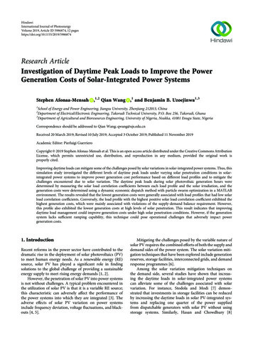
6International Journal of PhotoenergyTable 4: Results of 2-tailed tests showing the solar load correlation coeﬃcients and P values of various load proﬁles (LPs) under average,abundant, and scarce solar resource conditions.AverageLPCoeﬃcientP valueAbundantCoeﬃcientScarceP valueCoeﬃcientP value0.016LP10.539 0.0070.558 0.0050.486 LP20.458 0.0240.476 0.0190.433 910.3130.0830.1360.701 Correlation is signiﬁcant at the 0.05 level (2-tailed). Correlation is signiﬁcant at the 0.01 level (2-tailed).110112100108Solar power absorbed (%)Power generation cost (%)1101061041021009890807060961020 30Average1020 30 1020 30AbundantScarceSolar penetration (%)LP1LP2LP3LP4Figure 3: Power generation costs for the 24 h DEDs of the variousload proﬁles (LPs) under average, abundant, and scarce solarresource conditions.PV) was 13,616.40/day, which is comparable to the 13,555/day reported in [27]. The detailed results of theoptimal 24 h DED of the thermal generation units usingPSO are reported in Table S3 (see the Supplementarymaterial). However, note that the focus of this study is notto introduce a new optimization algorithm but rather toimplement an existing optimization algorithm to investigatethe diﬀerent levels of daytime peak loads under varyingsolar penetration conditions in solar-integrated powersystems in order to improve the power generation cost andmitigate the challenges related to solar variation.4. Results and DiscussionThe results of the power generation costs of the 24 h DED forvarious load proﬁles (LPs) are presented as percentages basedon a reference case (i.e., the initial load proﬁle, LP1) in whichthere was no solar PV in the DED (Figure 3). As shown inFigure 3, the power generation costs decreased with increasing solar penetration for LP2, LP3, and LP4.This reduction in the generation cost with increasingsolar penetration can be attributed to the continuous displacement of the thermal generation units with marginallyhigher generation costs than the solar PV as a result of the501020Average30102030102030AbundantScarceSolar penetration (%)LP3LP4LP1LP2Figure 4: Solar power absorption levels for the 24 h DEDs of theload proﬁles (LPs) under average, abundant, and scarce solarresource conditions.Table 5: Load factors of various load proﬁles (LPs).LP1LP2LP3LP40.7530.7920.8360.859solar power absorbed (Figure 4) [28]. Additionally, LP4,which had the lowest solar load correlation coeﬃcient, exhibited the lowest generation costs under average solar resourceconditions (Table 4).The minimum generation cost associated with LP4 wassupported by the results of several other studies that haveshown that load proﬁle ﬂattening can improve the generationcosts of solar-integrated power systems [29, 30]. As a conﬁrmation, the load factors, which are indicators of the ﬂatnessof the LPs, were estimated for the various LPs (Table 5)[31]. The high load factor of LP4, which was greater thanthose of the other load proﬁles, was also consistent with theresults obtained above.However, at the 10% and 20% solar penetration levelsunder abundant solar resource conditions, LP3, which hada higher positive solar load correlation coeﬃcient than LP4,

International Journal of Photoenergy7140000160000Power generation cost ( /h)Power generation cost ( 000080000600004000020000200000 2 4 6 8 10 12 14 16 18 20 22 24Time (h)LP1LP20 2 4 6 8 10 12 14 16 18 20 22 24Time (h)LP1LP2LP3LP4(a)(b)55000Power generation cost ( /h)Power generation cost ( 000300000 2 4 6 8 10 12 14 16 18 20 22 24Time (h)LP1LP20 2 4 6 8 10 12 14 16 18 20 22 24Time ower generation cost ( /h)Power generation cost ( 5000400003500030000250000 2 4 6 8 10 12 14 16 18 20 22 24Time (h)LP1LP2LP3LP4(e)0 2 4 6 8 10 12 14 16 18 20 22 24Time (h)LP1LP2LP3LP4(f)Figure 5: Hourly power generation costs for the 24 h DEDs of the load proﬁles (LPs) under (a) 10% average, (b) 30% average, (c) 10%abundant, (d) 30% abundant, (e) 10% scarce, and (f) 30% scarce solar penetration levels and resource conditions.exhibited the best generation cost performance amongthe various load proﬁles. This inconsistency is likelyrelated to the changes in the solar load correlation coefﬁcient of LP4 from a negative to a positive value(Table 4). According to Chaiamarit and Nuchprayoon[18], variable RE sources such as solar PV have a timevarying impact on system performance and can lead tochanges in the generation cost performance, such as thoseobserved for LP3 and LP4, under average and abundant solarresource conditions.

International Journal of Photoenergy2200220020002000Net-load (MW)Net-load (MW)8180016001400120018001600140012001000100002468 10 12 14 16 18 20 22 24Time (h)LP1LP202LP3LP4468 10 12 14 16 18 20 22 24Time (h)LP1LP2LP3LP4(a)(b)Figure 6: Net load curves of the load proﬁles (LPs) for (a) 10% and (b) 30% solar penetration levels and abundant solar resource conditions.1602400Power generation cost (%)22002000Load (MW)1800160014001200100014012010080800606000246810 12 14 16 18 20 22 241020 30AverageTime (h)Load profileNet-load curveLP5LP1Figure 7: Twenty-four-hour load proﬁle and net load curve of LP5at 30% solar penetration under abundant solar resource conditions.Table 6: Results of 2-tailed tests showing the solar load correlationcoeﬃcients and P values of LP5 under average, abundant, and scarcesolar resource conditions.AverageAbundantScarceCoeﬃcient P value Coeﬃcient P value Coeﬃcient P value0.652 0.0010.673 10 20 30 10 20 30AbundantScarceSolar penetration (%)0.0010.567 0.004Correlation is signiﬁcant at the 0.01 level (2-tailed).Moreover, LP1 (with the highest positive solar loadcorrelation coeﬃcient) exhibited the worst generationcosts, characterized by surges in most cases. Studies haveshown that the absorption of solar power can shift peakloads to other periods of the day when solar power diminishes [2, 15]. This possible load shift might have exacerbated the already existing peak at 20 h, making itimpossible for the dispatchable generation units to rampFigure 8: Power generation costs of the 24 h DED for LP5 and LP1under average, abundant, and scarce solar resource conditions.up to meet the rising load demand from 19 h to 20 hand violating the supply-demand balance requirement.Consequently, the penalty factor adopted in this studyresulted in the highest generation costs for LP1, whichwas characterized by surges (Figure 5).This ﬁnding indicates that LPs with high daytime peakloads could lead to operational challenges during the eveningload peaks in systems where dispatchable generation units donot have adequate ramping capability and can have adverseeﬀects on generation costs. Moreover, LPs with evening loadpeaks are common and typically characterize residential consumption patterns [9, 16, 32]. Therefore, in the utilization ofgrid-integrated solar PV, taking precautionary measures during evening load peaks in power systems with high daytimepeak loads could become necessary. In this regard, the lackof supply-demand balance requirement violations in the

International Journal of Photoenergy9Power generation cost ( /h)Power generation cost ( 015000010000050000000 2 4 6 8 10 12 14 16 18 20 22 24Time (h)(a)0 2 4 6 8 10 12 14 16 18 20 22 24Time (h)(b)Figure 9: Hourly power generation costs of the 24 h DED for LP5 at 30% solar penetration under (a) abundant and (b) scarce solar resourceconditions.Power generation cost Load profileFigure 10: Power generation costs of the 24 h DEDs of the variousload proﬁles (LPs) at 40% solar penetration under abundant solarresource conditions.other LPs suggests that adopting demand-side management(DSM) techniques to reduce evening load peaks could solvethe ramping problem.However, at 30% solar penetration under abundant solarresource conditions, LP1 exhibited the most cost-eﬀectiveload proﬁle among the various load proﬁles, with a generation cost of 96.36%. This observation is likely related to themore extensive eﬀects of high solar power penetration onthe characteristics of LP1 and LP2 than on those of LP3and LP4. Thus, Figures 6(a) and 6(b) illustrate the potentialimpact of solar PV on the LPs as the solar penetrationincreases from 10% to 30% using the net load concept[13, 18]. The ﬁgures show that there was a notable reduction in the daytime loads, particularly the daytime peakloads of LP1 and LP2 compared to those of LP3 andLP4, as the solar penetration increased from 10% to30%, which agrees with the previous results.Similarly, the obvious changes in the characteristics ofLP2 are attributable to the considerable reduction in the generation cost from 97.5% to 96.67% as the solar penetrationincreased from 20% to 30% under abundant solar conditions.Conversely, the generation cost of LP3 increased by 0.24% asthe solar penetration increased from 20% to 30%. The resultsobtained under the high solar penetration condition agreedwith those in previous studies [8, 10, 11], which found thatimproving the daytime loads improved the generation costsof solar-integrated power systems.Moreover, the diﬀerent eﬀects of solar PV on variousLPs as the solar penetration increased from 10% to 30%under abundant solar conditions aligned with those ofother studies, in which a signiﬁcant share of variablerenewable sources in power systems altered the originalload characteristics [15–18].Additionally, the results of violating the supplydemand balance requirements under relatively low solarpenetration conditions (i.e., 10% penetration) in LP4 dueto the inadequate ramping capability of the dispatchablegeneration units agreed with the ﬁndings in Ref. [16].Notably, Ref. [16] found that even low penetration levelsof solar PV could result in a high demand for the generation system ramping capability. It is worth noting that, at10% solar penetration under scarce solar conditions, thesupply-demand balance requirements were violated inLP2 due to ramping challenges in the generation units(Figure 5(e)). This observation could be related to undulations in the scarce solar resource condition proﬁle compared to the bell-shaped average and abundant solarresource condition proﬁles (Figure 2).Likewise, the undulating shape of the scarce solarresource condition proﬁle may be the reason for the relativelyirregular power generation cost performance observed forthe vario

tems have not clearly provided this key information. Thus, the main contribution of this study is to improve the genera-tion costs of solar-integrated power systems by investigating the generation cost performance of load proﬁles at various levels of daytime peak loads under varying solar penetration