Transcription
2This work is licenced under the Creative Commons Attribution-Non-Commercial-Share Alike 2.0 UK:England & Wales License. To view a copy of this licence, visit / or send a letter to Creative Commons, 171 Second Street, Suite 300, San Francisco, California 94105, USA.
Quantum Mechanics INiels WaletMarch 23, 2010
2
Contents1Introduction1.1 Black-body radiation1.2 Photo-electric effect .1.3 Hydrogen atom . . .1.4 Wave particle duality1.5 Uncertainty . . . . .1.6 Tunneling . . . . . .33466772Concepts from classical mechanics2.1 Conservative fields . . . . . . . . . . . . . . . . . . . . . . . . . . . . . . . . . . . . . . . . . .2.2 Energy function . . . . . . . . . . . . . . . . . . . . . . . . . . . . . . . . . . . . . . . . . . . .2.3 Simple example . . . . . . . . . . . . . . . . . . . . . . . . . . . . . . . . . . . . . . . . . . . .999103The Schrödinger equation3.1 The state of a quantum system . . . . . . . . . . . . . . . . . . . . . . . . . . . . . . . . . . .3.2 Operators . . . . . . . . . . . . . . . . . . . . . . . . . . . . . . . . . . . . . . . . . . . . . . .3.3 Analysis of the wave equation . . . . . . . . . . . . . . . . . . . . . . . . . . . . . . . . . . . .111113134Bound states of the square well4.1 B2 0 . . . . . . . . . . . . . . . . . . . . . . . . . . . . . . . .4.2 A2 0 . . . . . . . . . . . . . . . . . . . . . . . . . . . . . . . .4.3 Some consequences . . . . . . . . . . . . . . . . . . . . . . . . .4.4 Lessons from the square well . . . . . . . . . . . . . . . . . . .4.5 A physical system (approximately) described by a square well.1517171720205Infinite well5.1 Zero of energy is arbitrary . . . . . . . . . . . . . . . . . . . . . . . . . . . . . . . . . . . . . .5.2 Solution . . . . . . . . . . . . . . . . . . . . . . . . . . . . . . . . . . . . . . . . . . . . . . . .2323236Scattering from potential steps and square barriers, etc.6.1 Non-normalisable wave functions . . . . . . . . . . . . . . . . . . . . . . . . . . . . . . . . .6.2 Potential step . . . . . . . . . . . . . . . . . . . . . . . . . . . . . . . . . . . . . . . . . . . . .6.3 Square barrier . . . . . . . . . . . . . . . . . . . . . . . . . . . . . . . . . . . . . . . . . . . . .272727297The Harmonic oscillator7.1 Dimensionless coordinates . . . . . .7.2 Behaviour for large y . . . . . . . .7.3 Taylor series solution . . . . . . . . .7.4 A few solutions . . . . . . . . . . . .7.5 Quantum-Classical Correspondence333334343636.3.
48CONTENTSThe formalism underlying QM8.1 Key postulates . . . . . . . . . . . . . . . . . . . . . . . . . .8.1.1 Wavefunction . . . . . . . . . . . . . . . . . . . . . .8.1.2 Observables . . . . . . . . . . . . . . . . . . . . . . .8.1.3 Hermitean operators . . . . . . . . . . . . . . . . . .8.1.4 Eigenvalues of Hermitean operators . . . . . . . . .8.1.5 Outcome of a single experiment . . . . . . . . . . .8.1.6 Eigenfunctions of x̂ . . . . . . . . . . . . . . . . . . .8.1.7 Eigenfunctions of p̂ . . . . . . . . . . . . . . . . . . .8.2 Expectation value of x̂2 and p̂2 for the harmonic oscillator .8.3 The measurement process . . . . . . . . . . . . . . . . . . .8.3.1 Repeated measurements . . . . . . . . . . . . . . . .393939394040414141414243Ladder operators9.1 Harmonic oscillators . . . . . . . . . . . . . . .9.2 The operators â and ↠. . . . . . . . . . . . . . .9.3 Eigenfunctions of Ĥ through ladder operations9.4 Normalisation and Hermitean conjugates . . .454545464710 Time dependent wave functions10.1 correspondence between time-dependent and time-independent solutions10.2 Superposition of time-dependent solutions . . . . . . . . . . . . . . . . . .10.3 Completeness and time-dependence . . . . . . . . . . . . . . . . . . . . . .10.4 Simple example . . . . . . . . . . . . . . . . . . . . . . . . . . . . . . . . . .10.5 Wave packets (states of minimal uncertainty) . . . . . . . . . . . . . . . . .10.6 computer demonstration . . . . . . . . . . . . . . . . . . . . . . . . . . . . .4949495050515211 3D Schrödinger equation11.1 The momentum operator as a vector .11.2 Spherical coordinates . . . . . . . . . .11.3 Solutions independent of θ and ϕ . . .11.4 The hydrogen atom . . . . . . . . . . .11.5 Now where does the probability peak?11.6 Spherical harmonics . . . . . . . . . .11.7 General solutions . . . . . . . . . . . .53535354555556579.
Chapter 1IntroductionOne normally makes a distinction between quantum mechanics and quantum physics. Quantum physicsis concerned with those processes that involve discrete energies, and quanta (such as photons). QuantumMechanics concerns the study of a specific part of quantum physics, those quantum phenomena describedby Schrödinger’s equation.Quantum physics plays a rôle on small (atomic and subatomic) scales (say length scales of the orderof 10 9 m) and below. You can see whether an expression has a quantum-physical origin as soon as itcontains Planck’s constant in one of its two guises 6.626 · 10 34 Js,h̄ h/2π 1.055 · 10 34 Js.h(1.1)Here we shall shortly review some of the standard examples for the break-down classical physics, whichcan be described by introducing quantum principles.1.1Black-body radiationIn the 19th century there was a lot of interest in thermodynamics. One of the areas of interest was therather contrived idea of a black body: a material kept at a constant temperature T, and absorbing anyradiation that falls on it. Thus all the light that it emits comes from its thermal energy, non of it is reflectedfrom other sources. A very hot metal is pretty close to this behaviour, since its thermal emission is veryFigure 1.1: An oven with a small window1
2CHAPTER 1. INTRODUCTIONFigure 1.2: The black-body spectrum as measured by COBE. ()much more intense than the environmental radiation. A slightly more realistic device is an oven with asmall window, which we need to observe the emitted radiation, see Fig. 1.1. The laws of thermal emissionhave been well tested on such devices. A very different example is the so-called 3 K microwave radiation(Penzias and Wilson, Nobel price 1978). This is a remnant from the genesis of our universe, and conformsextremely well to the black-body picture, as has been shown by the recent COBE experiment, see Fig. 1.2.The problem with the classical (Rayleigh-Jeans) law for black-body radiation is that it does suggestemission of infinite amounts of energy, which is clearly nonsensical. Actually it was for the description ofthis problem Planck invented Planck’s constant! Planck’s law for the energy density ate frequency ν fortemperature T is given by8πhν3ρ(ν, T ) 3 hν/kT.(1.2)c e 1The interpretation of this expression is that light consists of particles called photons, each with energy hν.If we look at Planck’s law for small frequencies hν kT, we find an expression that contains nofactors h (Taylor series expansion of exponent)ρ(ν, T ) 8πν2 kT.c3(1.3)This is the Rayleigh-Jeans law as derived from classical physics. If we integrate these laws over all frequencies we findZ 8π 5 k4 4T(1.4)dνρ(ν, T ) E 15c3 h30for Planck’s law, and infinity for the Rayleigh-Jeans law. The T 4 result has been experimentally confirmed,and predates Planck’s law.1.2Photo-electric effectWhen we shine a lamp on a metal surface, electrons escape the surface. This is a simple experimental fact,that can easily be demonstrated. The intreaguing point is that it takes a minimum frequency of light toremove electrons from a metal, and different metals require different minimal frequencies. Intensity playsno rôle in the threshold.The explanation for this effect is due to Einstein (actually he got the Nobel price for this work, sincehis work on relativity was too controversial). Suppose once again that light is made up from photons.
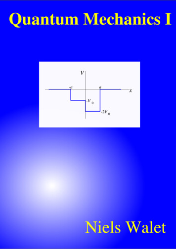
1.2. PHOTO-ELECTRIC EFFECT3Rayleigh-JeansPlanck’s law2-25-3ρ (10 Jsm )31002040608010010ν (10 Hz)Figure 1.3: A comparison between the Rayleigh-Jeans and Planck’s lawFigure 1.4: The photo-electric effect, where a single photon removes an electron from a metal.
4CHAPTER 1. INTRODUCTIONFigure 1.5: The Bohr model of the hydrogen atom, where a particle wave fits exactly onto a Keppler orbit.Assume further that the electrons are bound to the metal by an energy EB . Since they need to absorb lightto gain enough energy to escape from the metal, and it is extremely unlikely that they absorb multiplephotons, the individual photons must satisfyhν EB .(1.5)Thus the minimal frequency is ν0 EB /h. This is based on the quantum nature of light.1.3Hydrogen atomThe classical picture of the hydrogen atom is planetary in nature: an electron moves in an Kepler orbitaround the proton. The problem is that there is a force acting on the electron, and accelerated chargesradiate (that is what a radio is based on). This allows the atom to loose energy in a continuous way,slowly spiraling down until the electron lies on the proton. Now experiment show that this is not thecase: There are a discrete set of lines in the light emitted by hydrogen, and the electron will never loose allits energy. The first explanation for this fact came from Niels Bohr, in the so-called old quantum theory,where one assumes that motion is quantised, and only certain orbits can occur. In this model the energyof the Balmer series of Hydrogen is given by En e24πe0 22π 2 me 1.h2 n2(1.6)Clearly this is of quantum origin again.1.4Wave particle dualityIf waves (light) can be particles (photons), can particles (electrons, etc.) be waves? de Broglie gave apositive answer to this question, and argued that for a particle with energy E and momentum pEp hν h/λ(1.7)(1.8)
1.5. UNCERTAINTY5Figure 1.6: A double-slit experimentFigure 1.7: The tunneling phenomenon, where a particle can sometimes be found at the othee side of abarrier.where ν and λ are the frequency and the wavelength, respectively. These are exactly the relations for aphoton.One way to show that this behaviour is the correct one is to do the standard double slit experiment.For light we know that we have constructive or destructive interference if the difference in the distancetraveled between two waves reaching the same point is a integer (integer plus one half) times the wavelength of the light. With particles we would normally expect them to travel through one or the other ofeach of the slits. If we do the experiment with a lot of particles, we actually see the well known double-slitinterference.1.5UncertaintyA wave of sharp frequency has to last infinitely long, and is thus completely delocalised. What doesthis imply for matter waves? One of the implications is the uncertainty relation between position andmomentum x p & 12 h̄.(1.9)This implies that the combined accuracy of a simultaneous measurement of position and momentum hasa minimum. This is not important in problems on standard scales, for the following practical reason.Suppose we measure the velocity of a particle of 1g to be 1 10 6 m/s. In that case we can measureits position no more accurate that 5 · 10 26 m, a completely outrageous accuracy (remember, this is 10 16times the atomic scale!)1.6TunnelingIn classical mechanics a billiard ball bounces back when it hits the side of the billiard. In the quantumworld it might actually ”tunnel” through. Let me make this a little clearer. Classically a particle moving inthe following potential would just be bouncing back and fourth between the walls. This can be easily seenfrom conservation of energy: The kinetic energy can not go negative, and the total energy is conserved.
6CHAPTER 1. INTRODUCTIONWhere the potential is larger than the total energy, the particle cannot go. In quantum mechanics this isdifferent, and particles can penetrate these classically forbidden regions, escaping from their cage.This is a wave phenomenon, and is related to the behaviour of waves in impenetrable media: ratherthan oscillatory solutions, we have exponentially damped ones, that allow for some penetration. Thisalso occurs in processes such as total reflection of light from a surface, where the tunneling wave is called“evanescent”.
Chapter 2Concepts from classical mechanicsBefore we discuss quantum mechanics we need to consider some concepts of classical mechanics, whichare fundamental to our understanding of quantum mechanics.2.1Conservative fieldsIn all our discussions I will only consider forces which are conservative, i.e., where the total energy is aconstant. This excludes problems with friction. For such systems we can split the total energy in a partrelated to the movement of the system, called the kinetic energy (Greek κινeιν to move), and a secondpart called the potential energy, since it describes the potential of a system to produce kinetic energy.An extremely important property of the potential energy is that we can derive the forces as a derivavtive of the potential energy, typically denoted by V (r ), asF ( V (r ), V (r ), V (r )). x y z(2.1)A typical example of a potential energy function is the one for a particle of mass m in the earth’sgravitationol field, which in the flat-earth limit is written as V (r ) mgz. This leads to a gravitationalforceF (0, 0, mg)(2.2)Of course when total energy is conserved, that doesn’t define the zero of energy. The kinetic energyis easily defined to be zero when the particle is not moving, but we can add any constant to the potentialenergy, and the forces will not change. One typically takes V (r ) 0 when the length of r goes to .2.2Energy functiondOf course the kinetic energy is 12 mv2 , with v ṙ dtr. The sum of kinetic and potential energy can bewritten in the formE 21 mv2 V (r ).(2.3)Actually, this form is not very convenient for quantum mechanics. We rather work with the so-calledmomentum variable p mv. Then the energy functional takes the formE 12p2 V (r ).m(2.4)The energy expressed in terms of p and r is often called the (classical) Hamiltonian, and will be shown tohave a clear quantum analog.7
82.3CHAPTER 2. CONCEPTS FROM CLASSICAL MECHANICSSimple exampleWe can define all these concepts (velocity, momentum, potential) in one dimensionas well as in threedimensions. Let us look at the example for a barrier 0 x aV (x) (2.5)V0 x aWe can’t find a solution for E less than 0 (no solution for v). For energy less then V0 the particles can moveleft or right from the barrier, with constant velocity, but will make a hard bounce at the barrier (sign of v isnot determined from energy). For energies higher than V0 particles can move from one side to the other,but will move slower if they are above the barrier.
Chapter 3The Schrödinger equation3.1The state of a quantum systemLet us first look at how we specify the state for a classical system. Once again, we use the ubiquitousbilliard ball. As any player knows, there are three important aspects to its motion: position, velocity andspin (angular momentum around its centre). Knowing these quantities we can in principle (no friction)predict its motion for all times. We have argued before that quantum mechanics involves an element ofuncertainty. We cannot predict a state as in classical mechanics, we need to predict a probability. Wewant to be able to predict the outcome of a measurement of, say, position. Since position is a continuousvariable, we cannot just deal with a discrete probability, we need a probability density, To understand thisfact look at the probability that we measure x to be between X and X X. If X is small enough, thisprobability is directly proportional to the length of the intervalP( X x X X ) P ( X ) X(3.1)Here P ( X ) is called the probability density. The standard statement that the total probability is onetranslates to an integral statement,Z dx P ( x ) 1(3.2)(Here I am lazy and use the lower case x where I have used X before; this a standard practice in QM.)Since probabilities are always positive, we require P ( x ) 0.Now let us try to look at some aspects of classical waves, and see whether they can help us to guesshow to derive a probability density from a wave equation. The standard example of a classical wave isthe motion of a string. Typically a string can move up and down, and the standard solution to the waveequation 21 2A(x,t) A( x, t)(3.3) x2c2 x2can be positive as well as negative. Actually the square of the wave function is a possible choice for theprobability (this is proportional to the intensity for radiation). Now let us try to argue what wave equationdescribes the quantum analog of classical mechanics, i.e., quantum mechanics.The starting point is a propagating wave. In standard wave problems this is given by a plane wave,i.e.,ψ A exp(i (kx ωt φ)).(3.4)This describes a wave propagating in the x direction with wavelength λ 2π/k, and frequency ν ω/(2π ). We interpret this plane wave as a propagating beam of particles. If we define the probabilityas the square of the wave function, it is not very sensible to take the real part of the exponential: theprobability would be an oscillating function of x for given t. If we take the complex function A exp(i (kx ωt φ)), however, the probability, defined as the absolute value squared, is a constant ( A 2 ) independent9
10CHAPTER 3. THE SCHRÖDINGER EQUATIONof x and t, which is very sensible for a beam of particles. Thus we conclude that the wave function ψ( x, t)is complex, and the probability density is ψ( x, t) 2 .Using de Broglie’s relationp h̄/λ,(3.5)we findp h̄k.(3.6)The other of de Broglie’s relations can be used to giveE hν h̄ω.(3.7)One of the important goals of quantum mechanics is to generalise classical mechanics. We shall attemptto generalise the relation between momenta and energy,E 12 mv2 p22m(3.8)to the quantum realm. Notice thath̄ ψ( x, t)i xh̄i ψ( x, t)h̄ωψ( x, t) tpψ( x, t) h̄kψ( x, t) Eψ( x, t) (3.9)Using this we can guess a wave equation of the form12m h̄ i x 2ψ( x, t) h̄i ψ( x, t). t(3.10)Actually using the definition of energy when the problem includes a potential,E 21 mv2 V ( x ) p2 V (x)2m(3.11)(when expressed in momenta, this quantity is usually called a ”Hamiltonian”) we find the time-dependentSchrödinger equationh̄i h̄2 2ψ( x, t).(3.12)ψ( x, t) V ( x )ψ( x, t) 22m x tWe shall only spend limited time on this equation. Initially we are interested in the time-independentSchrödinger equation, where the probability ψ( x, t) 2 is independent of time. In order to reach this simplification, we find that ψ( x, t) must have the formψ( x, t) φ( x )e iEt/h̄ .(3.13)If we substitute this in the time-dependent equation, we get (using the product rule for differentiation) e iEt/h̄h̄2 d2φ( x ) e iEt/h̄ V ( x )φ( x ) Ee iEt/h̄ φ( x ).2m dx2(3.14)Taking away the common factor e iEt/h̄ we have an equation for φ that no longer contains time, the timeindepndent Schrödinger equationh̄2 d2φ( x ) V ( x )φ( x ) Eφ( x ).(3.15)2m dx2The corresponding solution to the time-dependent equation is the standing wave (3.13).
3.2. OPERATORS3.211OperatorsNotice that in deriving the wave equation we replaced the number p or k by a differential acting onthe wave function. The energy (or rather the Hamiltonian) was replaced by an ”operator”, which whenmultiplied with the wave function gives a combination of derivatives of the wave function and functionmultiplying the wave function, symbolically written asĤψ( x, t) h̄2 2ψ( x, t) V ( x )ψ( x, t).2m x2(3.16)This appearance of operators (often denoted by hats) where we were used to see numbers is one of thekey features of quantum mechanics.3.3Analysis of the wave equationOne of the important aspects of the Schrödinger equation(s) is its linearity. For the time independentSchrödinger equation, which is usually called an eigenvalue problem, the only consequence we shallneed here, is that if φ( x ) is a eigen function (a solution for Ei ) of the Schrödinger equation, so is Aφi ( x ).This is useful in defining a probability, since we would likeZ A 2 φi ( x ) 2 dx 1(3.17)Given φi ( x ) we can thus use this freedom to ”normalise” the wave function! (If the integral over φ( x ) 2is finite, i.e., if φ( x ) is “normalisable”.)Example 3.1:As an example suppose that we have a Hamiltonian that has the function ψi ( x ) e xeigen function. This function is not normalised sinceZ φi ( x ) 2 dx π.2 /2as(3.18)The normalised form of this function is21e x /2 .(π )1/4(3.19)We need to know a bit more about the structure of the solution of the Schrödinger equation – boundaryconditions and such. Here I shall postulate the boundary conditions, without any derivation.1. φ( x ) is a continuous function, and is single valued.R 2. φ( x ) 2 dx must be finite, so that φ( x ) 22 ψ ( x ) dxP( x ) R is a probability density.3. φ( x )/ x is continuous except where V ( x ) has an infinite discontinuity.(3.20)
12CHAPTER 3. THE SCHRÖDINGER EQUATION
Chapter 4Bound states of the square wellOne of the simplest potentials to study the properties of is the so-called square well potential, V 0 V0 x a. x a(4.1)We define three areas, from left to right I, II and III. In areas I and III we have the Schrödinger equationh̄2 d2ψ( x ) Eψ( x )2m dx2(4.2)h̄2 d2ψ( x ) ( E V0 )ψ( x )2m dx2(4.3) whereas in area II we have the equation Solution to a few ODE’s. In this class we shall quite often encounter the ordinary differential equationsd2f ( x ) α2 f ( x )dx2(4.4)f ( x ) A1 cos(αx ) B1 sin(αx ) C1 eiαx D1 e iαx ,(4.5)d2g ( x ) α2 g ( x )dx2(4.6)g( x ) A2 cosh(αx ) B2 sinh(αx ) C2 eαx D2 e αx .(4.7)which has as solutionandwhich has as solutionLet us first look at E 0. In that case the equation in regions I and I I I can be written asd22mψ( x ) 2 Eψ( x ) k2 ψ( x ),dx2h̄13(4.8)
14CHAPTER 4. BOUND STATES OF THE SQUARE WELLFigure 4.1: The square well potentialwheresk 2mh̄2E.(4.9)The solution to this equation is a sum of sines and cosines of kx, which cannot be normalised: Writeψ I I I ( x ) A cos(kx ) B sin(kx ) (A, B, complex) and calculate the part of the norm originating in regionI I I,Z a ψ( x ) 2 dx Z a A 2 cos2 kx B 2 sin2 kx 2 ( AB ) sin(kx ) cos(kx )dxlim NN Z 2π/ka A 2 cos2 (kx ) B 2 sin2 (kx )lim N ( A 2 /2 B 2 /2) .N (4.10)We also find that the energy cannot be less than V0 , since we vannot construct a solution for thatvalue of the energy. We thus restrict ourselves to V0 E 0. We writeE h̄2 k2,2mE V0 h̄2 κ 2.2m(4.11)The solutions in the areas I and III are of the form (i 1, 3)ψ( x ) Ai ekx Bi e kx .(4.12)In region II we have the oscillatory solutionψ( x ) A2 cos(κx ) B2 sin(κx ).(4.13)Now we have to impose the conditions on the wave functions we have discussed before, continuity ofψ and its derivatives. Actually we also have to impose normalisability, which means that B1 A3 0(exponentially growing functions can not be normalised). As we shall see we only have solutions atcertain energies. Continuity implies thatA1 e ka B1 eka A2 cos(κa) B2 sin(κa)ka ka A2 cos(κa) B2 sin(κa)kakaA3 e B3 ekA1 e kB1 ekakA3 e kB3 e ka κA2 sin(κa) κB2 cos(κa) κA2 sin(κa) κB2 cos(κa)(4.14)
4.1. B2 015Tactical approach: We wish to find a relation between k and κ (why?), removing as manby of the constantsA and B. The trick is to first find an equation that only contains A2 and B2 . To this end we take the ratioof the first and third and second and fourth equation:k k κ [ A2 sin(κa) B2 cos(κa)]A2 cos(κa) B2 sin(κa)κ [ A2 sin(κa) B2 cos(κa)]A2 cos(κa) B2 sin(κa)(4.15)We can combine these two equations to a single one by equating the right-hand sides. After deleting thecommon factor κ, and multiplying with the denominators we find[ A2 cos(κa) B2 sin(κa)][ A2 sin(κa) B2 cos(κa)] [ A2 sin(κa) B2 cos(κa)][ A2 cos(κa) B2 sin(κa)],(4.16)A2 B2 0(4.17)which simplifies toWe thus have two families of solutions, those characterised by B2 0 and those that have A2 0.4.1B2 0In the first case we read off that A1 B3 , and we find that k and κ are related byka κa tan κa.(4.18)qThis equation can be solved graphically. Use k κ 2 κ02 , with κ02 2m2 V0 , and find that there ish̄always at least one solution of this kind, no matter how small V0 ! In the middle region all these solutionsbehave like sines, and you will be asked to show that the solutions are invariant when x goes to x. (Wesay that these functions are even.)4.2A2 0In this case A1 B3 , and the relation between k and κ is modified toka κa cot κa.(4.19)From the graphical solution, in Fig. 4.3 we see that this type of solution only occurs for κ0 a greater thanπ/2. In the middle region all these solutions behave like sines, and you will be asked to show that thesolutions turn into minus themselves when x goes to x. (We say that these functions are odd.)4.3Some consequencesThere are a few good reasons why the dependence in the solution is on ka, κa and κ0 a: These are alldimensionless numbers, and mathematical relations can never depend on parameters that have a dimension! For the case of the even solutions, the ones with B2 0, we find that the number of bound states isdetermined by how many times we can fit 2π into κ0 a. Since κ0 is proportional to (the square root) of V0 ,we find that increasing V0 increases the number bound states, and the sameqhappens when we increasethe width a. Rewriting κ0 a slightly we find that the governing parameter is2mV a2 ,h̄2 0so that a factor oftwo change in a is the same as a factor four change in V0 .If we put the two sets of solutions on top of one another we see that after every even solution we getan odd solution, and vice versa.There is always at least one solution (the lowest even one), but the first odd solution only occurs whenκ0 a π
16CHAPTER 4. BOUND STATES OF THE SQUARE WELL10κa tanκaκ0a 1κ0a 550-5024κa6810Figure 4.2: The graphical solution for the even states of the square well.
4.3. SOME CONSEQUENCES1710κa cotκaκ0a 1κ0a 550-5024κa6810Figure 4.3: The graphical solution for the odd states of the square well.
18CHAPTER 4. BOUND STATES OF THE SQUARE WELL4.4Lessons from the square wellThe computer demonstration showed the following features:1. If we drop the requirement of normalisability, we have a solution to the TISE at every energy. Onlyat a few discrete values of the energy do we have normalisable states.2. The energy of the lowest state is always higher than the depth of the well (uncertainty principle).3. Effect of depth and width of well. Making the well deeper gives more eigen functions, and decreasesthe extent of the tail in the classically forbidden region.4. Wave functions are oscillatory in classically allowed, exponentially decaying in classically forbiddenregion.5. The lowest state has no zeroes, the second one has one, etc. Normally we say that the nth state hasn 1 “nodes”.6. Eigen states (normalisable solutions) for different eigen values (energies) are orthogonal.4.5A physical system (approximately) described by a square wellAfter all this tedious algebra, let us look at a possible physical realisation of such a system. In order to dothat, I shall have to talk a little bit about semi-conductors. A semiconductor is a quantum system wherethe so-called valence electrons completely fill a valence band, and are separated by a gap from a set of freestates in a conduction band. These can both be thought of a continuous set of quantum states. The energydifference between the valence and conduction bands is different for different semi-conductors. This canbe used in so-called quantum-well structures, where we sandwich a thin layer of, e.g., GaAs between verythick layers of GaAlAs.Since the gap energy is a lot smaller for GaAs than for GaAlAs, we get the effect of a small square well(in both valence and conduction bands). The fact that we can have a few occupied additional levels in thevalence, and a few empty levels in the conduction band can be measured.The best way to do this, is to shine light on these systems, and see for which frequency we can creata transition (just like in atoms). Phil Dawson has been so kind to provide me with a few slides of suchexperiments.
4.5. A PHYSICAL SYSTEM (APPROXIMATELY) DESCRIBED BY A SQUARE WELLFigure 4.4: A schematic representation of a quantum well19
20CHAPTER 4. BOUND STATES OF THE SQUARE WELL
Chapter 5Infinite well5.1Zero of energy is arbitraryThe normal definition of a potential energy is somewhat arbitrary. Consider where a potential comesfrom: It appears when the total energy (potential plus kinetic) is constant. But if something is constant,we can add a number to it, and it is still constant! Thus whether we define the gravitational potentialat the surface of the earth to be 0 or 100 J does not matter. Only dif
Concepts from classical mechanics Before we discuss quantum mechanics we need to consider some concepts of classical mechanics, which are fundamental to our understanding of quantum mechanics. 2.1 Conservative fields In all our discussions I will only consider forces which are conservative, i.e., where the total energy is a constant.