Transcription
Proceedings of the 2019 Winter Simulation ConferenceN. Mustafee, K.-H.G. Bae, S. Lazarova-Molnar, M. Rabe, C. Szabo, P. Haas, and Y.-J. Son, eds.ARRAY-RQMC FOR OPTION PRICING UNDER STOCHASTIC VOLATILITY MODELSAmal Ben AbdellahPierre L’EcuyerFlorian PuchhammerDépartement d’Informatique et de Recherche OpérationnellePavillon Aisenstadt, Université de MontréalC.P. 6128, Succ. Centre-VilleMontréal (Québec), H3C 3J7, CANADAABSTRACTArray-RQMC has been proposed as a way to effectively apply randomized quasi-Monte Carlo (RQMC)when simulating a Markov chain over a large number of steps to estimate an expected cost or reward. Themethod can be very effective when the state of the chain has low dimension. For pricing an Asian optionunder an ordinary geometric Brownian motion model, for example, Array-RQMC can reduce the varianceby factors in the millions. In this paper, we show how to apply this method and we study its effectivenessin case the underlying process has stochastic volatility. We show that Array-RQMC can also work verywell for these models, even if it requires RQMC points in larger dimension. We examine in particular thevariance-gamma, Heston, and Ornstein-Uhlenbeck stochastic volatility models, and we provide numericalresults.1INTRODUCTIONQuasi-Monte Carlo (QMC) and randomized QMC (RQMC) methods can improve efficiency significantlywhen estimating an integral in a moderate number of dimensions, but their use for simulating Markovchains over a large number of steps has been limited so far. The array-RQMC method, developed for thatpurpose, has been shown to work well for some chains having a low-dimensional state. It simulates anarray of n copies of the Markov chain so that each chain follows its exact distribution, but the copies are notindependent, and the empirical distribution of the states at any given step of the chain is a “low-discrepancy”approximation of the exact distribution. At each step, the n chains (or states) are matched one-to-one to aset of n RQMC points whose dimension is the dimension of the state plus the number of uniform randomnumbers required to advance the chain by one more step. The first coordinates of the points are used tomatch the states to the points and the other coordinates provide the random numbers needed to determine thenext state. When the chains have a large-dimensional state, the dimension used for the match can be reducedvia a mapping to a lower-dimensional space. Then the matching is performed by sorting both the pointsand the chains. When the dimension of the state exceeds 1, this matching is done via a multivariate sort.The main idea is to evolve the array of chains in a way that from step to step, the empirical distribution ofthe states keeps its low discrepancy. For further details on the methodology, sorting strategies, convergenceanalysis, applications, and empirical results, we refer the reader to Lécot and Tuffin (2004), Demers et al.(2005), L’Ecuyer et al. (2006), L’Ecuyer et al. (2007), L’Ecuyer et al. (2008), El Haddad et al. (2008),L’Ecuyer et al. (2009), El Haddad et al. (2010), Dion and L’Ecuyer (2010), L’Ecuyer and Sanvido (2010),Gerber and Chopin (2015), L’Ecuyer et al. (2018), and the other references given there.The aim of this paper is to examine how Array-RQMC can be applied for option pricing under astochastic volatility process such as the variance gamma, Heston, and Ornstein-Uhlenbeck models. We978-1-7281-3283-9/19/ 31.00 2019 IEEE440
Ben Abdellah, L’Ecuyer, and Puchhammerexplain and compare various implementation alternatives, and report empirical experiments to assess the(possible) gain in efficiency and convergence rate. A second objective is for the WSC community to becomebetter aware of this method, which can have numerous other applications.Array-RQMC has already been applied for pricing Asian options when the underlying process evolvesas a geometric Brownian motion (GBM) with fixed volatility (L’Ecuyer et al. 2009; L’Ecuyer et al. 2018).In that case, the state is two-dimensional (it contains the current value of the GBM and its running average)and a single random number is needed at each step, so the required RQMC points are three-dimensional.In their experiments, L’Ecuyer et al. (2018) observed an empirical variance of the average payoff thatdecreased approximately as O(n 2 ) for Array-RQMC, in a range of reasonable values of n, compared withO(n 1 ) for independent random points (Monte Carlo). For n 220 (about one million chains), the varianceratio between Monte Carlo and Array-RQMC was around 2 to 4 millions.In view of this spectacular success, one wonders how well the method would perform when theunderlying process is more involved, e.g., when it has stochastic volatility. This is relevant becausestochastic volatility models are more realistic than the plain GBM model (Madan and Seneta 1990; Madanet al. 1998). Success is not guaranteed because the dimension of the required RQMC points is larger. Forthe Heston model, for example, the RQMC points must be five-dimensional instead of three-dimensional,because the state has three dimensions and we need two uniform random numbers at each step. It is uncleara priori if there will be any significant variance reduction for reasonable values of n.The remainder is organized as follows. In Section 2, we state our general Markov chain model andprovide background on the Array-RQMC algorithm, including matching and sorting strategies. In Section3, we describe our experimental setting, and the types of RQMC point sets that we consider. Then westudy the application of Array-RQMC under the variance-gamma model in Section 4, the Heston modelin Section 5, and the Ornstein-Uhlenbeck model in Section 6. We end with a conclusion.2BACKGROUND: MARKOV CHAIN MODEL, RQMC, AND ARRAY-RQMCThe option pricing models considered in this paper fit the following framework, which we use to summarizethe Array-RQMC algorithm. We have a discrete-time Markov chain {X j , j 0} defined by a stochasticrecurrence over a measurable state space X :X0 x0 ,andX j ϕ j (X j 1 , U j ),j 1, . . . , τ,where x0 X is a deterministic initial state, U1 , U2 , . are independent random vectors uniformly distributedover the d-dimensional unit cube (0, 1)d , the functions ϕ j : X (0, 1)d X are measurable, and τ is afixed positive integer (the time horizon). The goal is:Estimateµy E[Y ],where Y g(Xτ )and g : X R is a cost (or reward) function. Here we have a cost only at the last step but in generalthere can be a cost function for each step and Y would be the sum of these costs (L’Ecuyer et al. 2008).Crude Monte Carlo estimates µ by the average Ȳn n1 n 1i 0 Yi , where Y0 , . . . ,Yn 1 are n independentrealizations of Y . One has E[Ȳn ] µy and Var[Ȳn ] Var[Y ]/n, assuming that E[Y 2 ] σy2 . Note that thesimulation of each realization of Y requires a vector V (U1 , . . . , Uτ ) of dτ independent uniform randomvariables over (0, 1), and crude Monte Carlo produces n independent replicates of this random vector.Randomized quasi-Monte Carlo (RQMC) replaces the n independent realizations of V by n dependentrealizations, which form an RQMC point set in dτ dimensions. That is, each Vi has the uniform distributionover [0, 1)dτ , and the point set Pn {V0 , .,Vn 1 } covers [0, 1)dτ more evenly than typical independentrandom points. With RQMC, Ȳn remains an unbiased estimator of µ, but its variance can be much smaller,and can converge faster than O(1/n) under certain conditions. For more details, see Dick and Pillichshammer(2010), L’Ecuyer and Lemieux (2000), L’Ecuyer (2009), L’Ecuyer (2018), for example. However, when dτis large, standard RQMC typically becomes ineffective, in the sense that it does not bring much variancereduction unless the problem has special structure.441
Ben Abdellah, L’Ecuyer, and PuchhammerArray-RQMC is an alternative approach developed specifically for Markov chains (L’Ecuyer et al. 2006;L’Ecuyer et al. 2008; L’Ecuyer et al. 2018). To explain how it works, let us first suppose for simplicity(we will relax it later) that there is a mapping h : X R, that assigns to each state a value (or score)which summarizes in a single real number the most important information that we should retain from thatstate (like the value function in stochastic dynamic programming). This h is called the sorting function.The algorithm simulates n (dependent) realizations of the chain “in parallel”. Let Xi, j denote the state ofchain i at step j, for i 0, . . . , n 1 and j 0, . . . , τ. At step j, the n chains are sorted by increasing orderof their values of h(Xi, j 1 ), the n points of an RQMC point set in d 1 dimensions are sorted by their firstcoordinate, and each point is matched to the chain having the same position in this ordering. Each chaini is then moved forward by one step, from state Xi, j 1 to state Xi, j , using the d other coordinates of itsassigned RQMC point. Then we move on to the next step, the chains are sorted again, and so on.The sorting function can in fact be more general and have the form h : X Rc for some small integerc 1. Then the mapping between the chains and the points must be realized in a c-dimensional space, i.e.,via some kind of c-dimensional multivariate sort. The RQMC points then have c d coordinates, and aresorted with the same c-dimensional multivariate sort based on their first c coordinates, and mapped to thecorresponding chains. The other d coordinates are used to move the chains ahead by one step. In practice,the first c coordinates of the RQMC points do not have to be randomized at each step; they are usuallyfixed and the points are already sorted in the correct order based on these coordinates.Some multivariate sorts are described and compared by El Haddad et al. (2008), L’Ecuyer et al. (2009),L’Ecuyer (2018). For example, in a multivariate batch sort, we select positive integers n1 , . . . , nc such thatn n1 . . . nc . The states are first sorted by their first coordinate in n1 packets of size n/n1 , then each packetis sorted by the second coordinate into n2 packets of size n/n1 n2 , and so on. The RQMC points are sortedin exactly the same way, based on their first c coordinates. In the multivariate split sort, we assume thatn 2e and we take n1 n2 · · · ne 2. That is, we first split the points in 2 packets based on the firstcoordinate, then split each packet in two by the second coordinate, and so on. If e c, after c splits weget back to the first coordinate and continue.Examples of heuristic sorting functions h : X R are given in (L’Ecuyer et al. 2008; L’Ecuyer et al.2018). Wächter and Keller (2008) and Gerber and Chopin (2015) suggested to first map the c-dimensionalstates to [0, 1]c and then use a space filling curve in [0, 1]c to map them to [0, 1], which provides a total order.Gerber and Chopin (2015) proposed to map the states to [0, 1]c via a component-wise rescaled logistictransformation, then order them with a Hilbert space-filling curve. See L’Ecuyer et al. (2018) for a moredetailed discussion. Under smoothness conditions, they proved that the resulting unbiased Array-RQMCestimator has o(1/n) variance, which beats the O(1/n) Monte Carlo rate.Algorithm 1 states the Array-RQMC procedure in our setting. Indentation delimits the scope of the“for” loops. For any choice of sorting function h, the average µ̂arqmc,n Ȳn returned by this algorithmis always an unbiased estimator of µ. An unbiased estimator of Var[Ȳn ] can be obtained by making mindependent realizations of µ̂arqmc,n and computing their empirical variance.Algorithm 1 : Array-RQMC Algorithm for Our Settingfor i 0, . . . , n 1 do Xi,0 x0 ;for j 1, 2, . . . , τ doSorting: Compute an appropriate permutation π j of the n chains, based onthe h(Xi, j 1 ), to match the n states with the RQMC points;Randomize afresh the RQMC points {U0, j , . . . , Un 1, j };for i 0, . . . , n 1 do Xi, j ϕ j (Xπ j (i), j 1 , Ui, j );return the average µ̂arqmc,n Ȳn (1/n) n 1i 0 g(Xi,τ ) as an estimate of µy .442
Ben Abdellah, L’Ecuyer, and Puchhammer3EXPERIMENTAL SETTINGFor all the option pricing examples in this paper, we have an asset price that evolves as a stochasticprocess {S(t), t 0} and a payoff that depends on the values of this process at fixed observation times0 t0 t1 t2 . tc T . More specifically, for given constants r (the interest rate) and K (the strikeprice), we consider an European option whose payoff isY Ye g(S(T )) e rT max(S(T ) K, 0)and a discretely-observed Asian option whose payoff isY Ya g(S̄) e rT max(S̄ K, 0)jS(t ) must be kept inwhere S̄ (1/c) cj 1 S(t j ). In this second case, the running average S̄ j (1/ j) 1the state of the Markov chain. The information required for the evolution of S(t) depends on the model andis given for each model in forthcoming sections. It must be maintained in the state. For the case where Sis a plain GBM, the state of the Markov chain at step j can be taken as X j (S(t j ), S̄ j ), a two-dimensionalstate, as was done in L’Ecuyer et al. (2009) and L’Ecuyer et al. (2018).In our examples, the states are always multidimensional. To match them with the RQMC points, wewill use a split sort, a batch sort, and a Hilbert-curve sort, and compare these alternatives. The Hilbertsort requires a transformation of the -dimensional states to the unit hypercube [0, 1] . For this, we use alogistic transformation defined by ψ(x) (ψ1 (x1 ), ., ψ (x )) [0, 1] for all x (x1 , . . . , x ) X , where!# 1"xj xj, j 1, ., ,ψ j (x j ) 1 exp x̄ j x jwith constants x̄ j µ j 2σ j and x j µ j 2σ j in which µ j and σ j are estimates of the mean and thevariance of the distribution of the jth coordinate of the state. In Section 4, we will also consider just takinga linear combination of the two coordinates, to map a two-dimensional state to one dimension.For RQMC, we consider(1) Independent points, which corresponds to crude Monte Carlo (MC);(2) Stratified sampling over the unit hypercube (Stratif);(3) Sobol’ points with a random linear matrix scrambling and a digital random shift(Sobol’ LMS);(4) Sobol’ points with nested uniform scrambling (Sobol’ NUS);(5) A rank-1 lattice rule with a random shift modulo 1 followed by a baker’s transformation(Lattice baker).The first two are not really RQMC points, but we use them for comparison. For stratified sampling, wedivide the unit hypercube into n k d congruent subcubes for some integer k 1, and we draw one pointrandomly in each subcube. For a given target n, we take k as the integer for which k d is closest to thistarget n. For the Sobol’ points, we took the default direction numbers in SSJ, which are from Lemieuxet al. (2004). The LMS and NUS randomizations are explained in Owen (2003) and L’Ecuyer (2009). Forthe rank-1 lattice rules, we used generating vectors found by Lattice Builder (L’Ecuyer and Munger 2016),using the P2 criterion with order-dependent weights (0.8)k for projections of order k.For each example, each sorting method, each type of point set, and each selected value of n, weran simulations to estimate Var[Ȳn ]. For the stratified and RQMC points, this variance was estimated byreplicating the RQMC scheme m 100 times independently. For a fair comparison with the MC varianceσy2 Var[Y ], for these point sets we used the variance per run, defined as nVar[Ȳn ]. We define the variancereduction factor (VRF) for a given method compared with MC by σy2 /(nVar[Ȳn ]). In each case, we fitteda linear regression model for the variance per run as a function of n, in log-log scale. We denote by β̂ theregression slope estimated by this linear model.443
Ben Abdellah, L’Ecuyer, and PuchhammerIn the remaining sections, we explain how the process {S(t), t 0} is defined in each case, how it issimulated. We show how we can apply Array-RQMC and we provide numerical results. All the experimentswere done in Java using the SSJ library (L’Ecuyer and Buist 2005; L’Ecuyer 2016).4OPTION PRICING UNDER A VARIANCE-GAMMA PROCESSThe variance-gamma (VG) model was proposed for option pricing by Madan and Seneta (1990) and Madan,Carr, and Chang (1998), and further studied by Fu et al. (1998), Avramidis et al. (2003), Avramidis andL’Ecuyer (2006), for example. A VG process is essentially a Brownian process for which the time clockruns at random and time-varying speed driven by a gamma process. The VG process with parameters(θ , σ 2 , ν) is defined as Y {Y (t) X(G(t)), t 0} where X {X(t), t 0} is a Brownian motion withdrift and variance parameters θ and σ 2 , and G {G(t), t 0} is a gamma process with drift and volatilityparameters 1 and ν, independent of X. This means that X(0) 0, G(0) 0, both B and G have independentincrements, and for all t 0 and δ 0, we have X(t δ ) X(t) Normal(δ θ , δ σ 2 ), a normal randomvariable with mean δ θ and variance δ σ 2 , and G(t δ ) G(t) Gamma(δ /ν, ν), a gamma random variablewith mean δ and variance δ ν. The gamma process is always non-decreasing, which ensures that the timeclock never goes backward. In the VG model for option pricing, the asset value follows the geometricvariance-gamma (GVG) process S {S(t), t 0} defined byS(t) S(0) exp [(r ω)t X(G(t))] ,where ω ln(1 θ ν σ 2 ν/2)/ν.To generate realizations of S̄ for this process, we must generate S(t1 ), . . . , S(tτ ), and there are manyways of doing this. With Array-RQMC, we want to do it via a Markov chain with a low-dimensionalstate. The running average S̄ j must be part of the state, as well as sufficient information to generatethe future of the path. A simple procedure for generating the path is to sample sequentially G(t1 ), thenY (t1 ) X(G(t1 )) conditional on G(t1 ), then G(t2 ) conditional on G(t1 ), then Y (t2 ) X(G(t2 )) conditionalon (G(t1 ), G(t2 ),Y (t1 )), and so on. We can then compute any S(t j ) directly from Y (t j ).It is convenient to view the sampling of (G(t j ), Y (t j )) conditional on (G(t j 1 ), Y (t j 1 )) as one step (stepj) of the Markov chain. The state of the chain at step j 1 can be taken as X j 1 (G(t j 1 ), Y (t j 1 ), S̄ j 1 ),so we have a three-dimensional state, and we need two independent uniform random numbers at each step,one to generate G(t j ) and the other to generate Y (t j ) X(G(t j )) given (G(t j 1 ), G(t j ),Y (t j 1 )), both byinversion. Applying Array-RQMC with this setting would require a five-dimensional RQMC point set ateach step, unless we can map the state to a lower-dimensional representation.However, a key observation here is that the distribution of the increment Y j Y (t j ) Y (t j 1 ) dependsonly on the increment j G(t j ) G(t j 1 ) and not on G(t j 1 ). This means that there is no need tomemorize the latter in the state! Thus, we can define the state at step j as the two-dimensional vectorX j (Y (t j ), S̄ j ), or equivalently X j (S(t j ), S̄ j ), and apply Array-RQMC with a four-dimensional RQMCpoint set if we use a two-dimensional sort for the states, and a three-dimensional RQMC point set if wemap the states to a one-dimensional representation (using a Hilbert curve or a linear combination of thecoordinates, for example). At step j, we generate j Gamma((t j t j 1 )/ν, ν) by inversion using auniform random variate U j,1 , i.e., via j Fj 1 (U j,1 ) where Fj is the cdf of the Gamma((t j t j 1 )/ν, ν)distribution, then Y j by inversion from the normal distribution with mean θ j and variance σ 2 j , using auniform random variate U j,2 . Algorithm 2 summarizes this procedure. The symbol Φ denotes the standardnormal cdf. We haveX j (Y (t j ), S̄ j ) ϕ j (Y (t j 1 ), S̄ j 1 ,U j,1 ,U j,2 )where ϕ j is defined by the algorithm. The payoff function is g(Xc ) S̄c S̄.With this two-dimensional state representation, if we use a split sort or batch, we need four-dimensionalRQMC points. With the Hilbert-curve sort, we only need three-dimensional RQMC points. We also tried asimple linear mapping h j : R2 R defined by h j (S(t j ), S̄ j ) b j S̄ j (1 b j )S(t j ) where b j ( j 1)/(τ 1).444
Ben Abdellah, L’Ecuyer, and PuchhammerAlgorithm 2 Computing X j (Y (t j ), S̄ j ) given (Y (t j 1 ), S̄ j 1 ), for 1 j τ.Generate U j,1 ,U j,2 Uniform(0, 1), independent; j Fj 1 (U j,1 ) Gamma((t j t j 1 )/ν, ν);Z j Φ 1 (U j,2 ) Normal(0,p1);Y (t j ) Y (t j 1 ) θ j σ j Z j ;S(t j ) S(0) exp[(r ω)t j Y (t j )];S̄ j [( j 1)S̄ j 1 S(t j )]/ j;At each step j, this h j maps the state X j to a real number h j (X j ), and we sort the states by increasing orderof their value of h j (X j ). It uses a convex linear combination of S(t j ) and S̄ j whose coefficients depend on j.The rationale for the (heuristic) choice of b j is that in the late steps (when j is near τ), the current averageS̄ j is more important (has more predictive power for the final payoff) than the current S(t j ), whereas in theearly steps, the opposite is true.We made an experiment with the following model parameters, taken from Avramidis and L’Ecuyer(2006): θ 0.1436, σ 0.12136, ν 0.3, r 0.1, T 240/365, τ 10, t j 24 j/365 for j 1, . . . , τ,K 100, and S(0) 100. The time unit is one year, the horizon is 240 days, and there is an observationtime every 24 days. The exact value of the expected payoff for the Asian option is µ 8.36, and the MCvariance per run is σy2 Var[Ya ] 59.40.arqmcTable 1: Regression slopes β̂ for log2 Var[µ̂n] vs log2 (n), and VRF compared with MC for n 220 ,denoted VRF20, for the Asian option under the VG model.SortSplit sortBatch sort(n1 n2 )Hilbert sort(with logisticmap)Linear mapsortPoint setsMCStratifSobol’ LMSSobol’ NUSLattice bakerMCStratifSobol’ LMSSobol’ NUSLattice bakerMCStratifSobol’ LMSSobol’ NUSLattice bakerMCStratifSobol’ LMSSobol’ NUSLattice 29779,86945,8541192115,216166,54168,739Table 1 summarizes the results. For each selected sorting method and point set, we report the estimatedarqmcslope β̂ for the linear regression model of log2 Var[µ̂n] as a function of log2 (n) obtained from m 100independent replications with n 2e for e 16, ., 20, as well as the variance reduction factors (VRF)observed for n 220 (about one million samples), denoted VRF20. For MC, the exact slope (or convergencerate) β is known to be β 1. We see from the table that Array-RQMC provides much better convergencerates (at least empirically), and reduces the variance by very large factors for n 220 . Interestingly, thelargest factors are obtained with the Sobol’ points combined with our heuristic linear map sort, although445
Ben Abdellah, L’Ecuyer, and PuchhammerMCStratifSobol’ LMSSobol’ NUSLattice bakerMCStratifSobol LMSSobol’ NUSLattice bakerMCStratifSobol LMSSobol’ NUSLattice bakerMCStratifSobol LMSSobol’ NUSLattice baker 10 10 10 10 20 20 20 20 30 30 30 301618log2 (n)2016182016log2 (n)1820161820log2 (n)log2 (n)arqmcFigure 1: Plots of empirical log2 Var[µ̂n] vs log2 (n) for various sorts and point sets, based on m 100independent replications. Left to right: split sort, batch sort, Hilbert sort, linear map sort.arqmcthe other sorts are also doing quite well. Figure 1 shows plots of log2 Var[µ̂n] vs log2 (n) for selectedsorts. It gives an idea of how well the linear model fits in each case.There are other ways of defining the steps of the Markov chain for this example. For example, one canhave one step for each Uniform(0, 1) random number that is generated. This would double the number ofsteps, from c to 2c. We generate 1 in the first step, Y (t1 ) in the second step, 2 in the third step, Y (t2 ) inthe fourth step, and so on. Generating a single uniform per step instead of two reduces by 1 the dimensionof the required RQMC point set. At odd step numbers, when we generate a j , the state can still be takenas (Y (t j 1 ), S̄ j 1 ) and we only need three-dimensional RQMC points, so we save one dimension. But ateven step numbers, we need j to generate Y (t j ), so we need a three-dimensional state (Y (t j 1 ), j , S̄ j 1 )and four-dimensional RQMC points. We tried this approach and it did not perform better than the onedescribed earlier, with two uniforms per step. It is also more complicated to implement.Avramidis et al. (2003), Avramidis and L’Ecuyer (2006) describe other ways of simulating the VGprocess, for instance Brownian and gamma bridge sampling (BGBS) and difference of gammas bridgesampling (DGBS). BGBS generates first G(tc ) then Y (tc ), then conditional on this it generates G(tc/2 )then Y (tc/2 ) (assuming that c is even), and so on. DGBS writes the VG process Y as a difference of twoindependent gamma processes and simulate both using the bridge idea just described: first generate thevalues of the two gamma processes at tc , then at tc/2 , etc. When using classical RQMC, these samplingmethods brings an important variance reduction compared with the sequential one we use here for ourMarkov chain. Combining them with Array-RQMC is impractical, however, because the dimension of thestate (the number of values that we need to remember and use for the sorting) grows up to about c, whichis much to high, and the implementation is much more complicated. Also, these methods are effectivewhen c is a power or 2 and t j jT /c, because then the conditional sampling for the gamma process isalways from a symmetrical beta distribution and there is an efficient inversion method for that (L’Ecuyerand Simard 2006), but they are less effective otherwise. For comparison, we made an experiment usingclassical RQMC with these methods for the same numerical example as given here, but with c 8 andc 16 instead of c 10, to have powers of 2, and t j jT /c. For Sobol’ LMS with n 220 , for d 16,the values of VRF20 for BGSS, BGBS, and DGBS were 85, 895, 550, respectively. For d 8, these valueswere 183, 1258, and 3405. The VRF20 values for Sobol’ LMS in table 1 and are much larger that these,showing that Array-RQMC can provide much larger variance reductions.For this VG model, we do not report results on the European option with Array-RQMC, because theMarkov chain would have only one step: We can generate directly G(tc ) and then Y (tc ). For this, ordinaryRQMC works well enough (L’Ecuyer 2018).446
Ben Abdellah, L’Ecuyer, and Puchhammer5OPTION PRICING UNDER THE HESTON VOLATILITY MODELThe Heston volatility model is defined by the following two-dimensional stochastic differential equation:dS(t) rS(t)dt V (t)1/2 S(t)dB1 (t),dV (t) λ (σ 2 V (t))dt ξV (t)1/2 dB2 (t),for t 0, where (B1 , B2 ) is a pair of standard Brownian motions with correlation ρ between them, r isthe risk-free rate, σ 2 is the long-term average variance parameter, λ is the rate of return to the meanfor the variance, and ξ is a volatility parameter for the variance. The processes S {S(t), t 0} andV {V (t), t 0} represent the asset price and the volatility, respectively, as a function of time. We willexamine how to estimate the price of European and Asian options with Array-RQMC under this model.Since we do not know how to generate (S(t δ ), V (t δ )) exactly from its conditional distribution given(S(t), V (t)) in this case, we have to discretize the time. For this, we use the Euler method with τ timesteps of length δ T /τ to generate a skeleton of the process at times w j jδ for j 1, . . . , τ, over [0, T ].For the Asian option, we assume for simplicity that the observation times t1 , . . . ,tc used for the payoff areall multiples of δ , so each of them is equal to some w j .arqmcTable 2: Regression slopes β̂ for log2 Var[µ̂n] vs log2 (n), and VRF compared with MC for n 220 ,denoted VRF20, for the Asian option under the Heston model.SortSplit sortBatch sortHilbert sort (withlogistic map)Point setsMCStratifSobol’ LMSSobol’ NUSLattice bakerMCStratifSobol’ LMSSobol’ NUSLattice bakerMCStratifSobol’ LMSSobol’ NUSLattice bakerEuropeanβ̂ VRF20-11-1.26103-1.59 44,188-1.46 30,616-1.50 26,772-11-1.2491-1.66 22,873-1.72 30,832-1.75 12,562-11-1.2643-1.14368-1.06277-1.12250Asianβ̂ .1149-0.8942Following Giles (2008), to reduce the bias due to the discretization, we make the change of variableW (t) eλt (V (t) σ 2 ), with dW (t) eλt ξV (t)1/2 dB2 (t), and apply the Euler method to (S,W ) instead of(S,V ). The Euler approximation scheme with step size δ applied to W givese ( jδ ) We (( j 1)δ ) eλ ( j 1)δ ξ (Ve (( j 1)δ )δ )1/2 Z j,2 .WRewriting it in terms of V by using the reverse identity V (t) σ 2 e λt W (t), and after some manipulations,we obtain the following discrete-time stochastic recurrence, which we will simulate by Array-RQMC:h iVe ( jδ ) max 0, σ 2 e λ δ Ve (( j 1)δ ) σ 2 ξ (Ṽ (( j 1)δ )δ )1/2 Z j,2 ,e jδ ) (1 rδ )S((e j 1)δ ) (Ve (( j 1)δ )δ )1/2 S((e j 1)δ )Z j,1 ,S(where (Z j,1 , Z j,2 ) is a pair of standard normals with correlation ρ. We generate this pairp from a pair (U j,1 ,U j,2 ) 1of independent Uniform(0, 1) variables via Z j,1 Φ (U j,1 ) and Z j,2 ρZ j,1 1 ρ 2 Φ 1 (U j,2 ). We447
Ben Abdellah, L’Ecuyer, and Puchhammerlog2 (Var)MCStratifSobol’ LMSSobol’ NUSLattice bakerMCStratifSobol’ LMSSobol’ NUSLattice baker 10 10 15 15 20 10 15 20 25 20 251618201816log2 (n)2016log2 (n) 101820log2 (n)MCStratifSobol’ LMSSobol’ NUSLattice bakerMCStratifSobol’ LMSSobol’ NUSLattice bakerlog2 (Var)MCStratifSobol’ LMSSobol’ NUSLattice baker 10MCStratifSobol’ LMSSobol’ NUSLattice baker 10 15 201618 20 15 25 20201816log2 (n)log2 (n)20161820log2 (n)arqmcFigure 2: Plots of empirical log2 Var[µ̂n] vs log2 (n) for various sorts and point sets, based on m 100independent re
The aim of this paper is to examine how Array-RQMC can be applied for option pricing under a stochastic volatility process such as the variance gamma, Heston, and Ornstein-Uhlenbeck models. We 978-1-7281-3283-9/19/ 31.00 2019 IEEE 440