WIXLIB

Outline of the TextFirst SemesterIn Chapter 1 the basics of the differential calculus are introduced, mostly in the context of polynomial functions and relations. In section four the derivatives of the trigonometric functions arefound using the differential triangle of Pascal.Chapter 2 discusses the concept of limit, techniques for calculating limits, including l’Hôpital’srule. We show that the sine function is differentiable (a fact postponed from chapter 1). Limitsat infinity and asymptotes are discussed. The point of the last section is the affirmation that afunction with derivative 0 everywhere in an interval is constant. This is always a difficult passagein the first calculus course, for the students see this as the tautology that a function with no changethroughout an interval ends up at the same value with which it started. So, the instructor hasto first convince the student that there is a real issue here. In class, I’ll do that by exhibitingthe Cantor function, which is almost always constant, but somehow gets from 0 to 1. Thenthe instructor must confess that the issue will not be joined, and instead this fundamental factwill be shown to follow from statements (intermediate value, existence of maxima for continuousfunctions) that, for some reason, are more intuitively obvious. I leave the strategy for doing thisto the instructor, and instead just lay down the minimal exposition.Chapter 3 covers the geometric significance of the first and second derivatives, optimization andgraph sketching,Chapter 4 introduces integration as the process reverse to differentiation, and extends this toseparable differential equations. This leads to the introduction of the exponential function as thesolution of dy/y rdx. I do not feel that it is necessary to discuss the general concept of inversefunctions to get from the exponential to the logarithm; the logarithm is simply what we use to finda if we know ea .Chapter 5 turns to Liebniz’ concept of integration as a method of accumulation, and shows (throughthe Fundamental theorem) that the Calculi of Newton and Liebniz are the same subject. This isfollowed by the application of integration to a variety of accumulation processes.Covering these first 5 chapters in one semester is a tall order. It may be that the course willend with the fundamental theorem, and that the second semester starts with the applications ofintegration. Alternatively, some sections of these first five chapters may be omitted.Second SemesterWe are now in a position to abstractly discuss inverse functions and the fact that a function withnonzero derivative in an interval has an inverse, leading to the introduction of many useful transcendental functions. This, together with the solution of general first order differential equations,is covered in Chapter 6.Chapter 7 covers the techniques of integration necessary to make use of a table of integrals: substitution, integration by parts and partial fractions. It is the intent of this text that from this pointon, students will use a table of integrals.vi

Chapter 8 begins with a brief review of l’Hôpital’s rule, as some instructors may prefer to coverthis in the second semester. Then Improper Integrals are covered as this material will be necessaryfor the next chapter.We begin Chapter 9 (Sequences and Series) with a more formal discussion of the Principle ofMathematical Induction (although it has already been used informally in several places in thetext), in connection with the definition of sequences by recursion. As the point of this chapter isto develop ways to approximate values of transcendental functions, the focus is to get to Taylorseries quickly. It also works to cover section 10.1 (on the Taylor formula with estimate) beforeChapter 9, to better motivate the discussion of series. The important thing is to emphasize that acalculation is not an approximation without some estimate of the error.Chapter 10 is a brief introduction to the simplest numerical methods; enough to give an idea ofhow the basic computer algorithms work.Chapter 11 covers materials on the conics and polar coordinates. Although this material is traditionally pre-calculus, it is necessary to review it before launching into mulit-variate calculus. Thestring properties of the conics are derived, and their optical properties are derived as differentialversions of the string properties.Chapter 12 covers the usual material on second order differential equations and basic harmonics. Many students will have already covered this in the physics classes, and in many cases this isdone at the beginning of the course on differential equations. Thus, this chapter may be omitted,particularly if Calculus is three quarters rather than three semesters.Third SemesterThe introduction to Vector Algebra (chapter 13) is motivated by geometry, the point being tocharacterize linear subspaces in two and three dimensions in a variety of ways.One of the central themes of this text is the study of particles in motion; we discuss the calculus ofvector-valued functions of a single variable (Chapter 14)in this context. Sections 2 and three coverthe differential geometry of curves in two and three dimensions, and section 4 provides a derivationof Kepler’s Laws of Planetary Motion from Newton’s Laws of Motion.Chapter 15 (Coordinates and Surfaces) covers the basic geometric tools of the several variablecalculus: change of coordinates in two and three variables, surfaces, and in particular, the normalforms of quadrics.Chapters 16 and 17 cover differentiation and integration in several variables. The differential of afunction is introduced as the linear function which best fits the given function near a base point.Applications of integrals are discussed in detail in two dimensions.Chapter 18 (Vector Calculus) is motivated as the study of fluids in motion, paralleling the themeof particles in motion for the single variable calculus. The basic forms (curl and divergence) areintroduced in this context. This leads to an interpretation that makes the fundamental theorems(Green, Stokes, Gauss) plausible. Here the emphasis is on the examples which show how to useand apply these theorems.vii

CALCULUS I, First SemesterI. Rate of Change, Tangent Line and Differentiation1.1 Newton’s CalculusEarly in his career, Isaac Newton wrote, but did not publish, a paper referred to as the tractof october 1666. This was his sole work purely on mathematics, and contained the fundamentalideas and techniques of the calculus. While writing (1684-87) the Principia Mathematica, thefundamental exposition of his mathematical physics of “the system of the world”, he reworkedand expanded these ideas and included them as part of this treatise. Newton’s central conceptionwas that of objects in motion. To Newton motion is described by the position and velocity of theparticle relative to a fixed coordinate system, as functions of time. These then are the fundamentalvariables: x, y, z, etc., and their velocities are denoted by ẋ, ẏ, ż, etc. Now, velocity is a measureof the rate of change of position (and acceleration, denoted ẍ, etc., is a rate of change of velocity),and what was needed was a means to express this relationship, and a process of deriving relationsamong the various velocities and accelerations from given relations among the variables. This isthe Calculus of Newton.Calculus, as it is presented today starts in the context of two variables, or measurable quantities,x, y, which are related in the sense that values of one of the variables determine values of the other.A function y f (x) is a rule which specifies this relation between the input or independent variablex and the output or dependent variable y. This may be given by a formula, a table, or a computeralgorithm; in fact, any set of rules which uniquely determine outputs for given inputs. The set ofallowable values for the input variable is called the domain of the function, and the set of outputs,the range. In our context both the domain and the range are sets of real numbers.An interval is the set of all real numbers between specified real numbers c and d. This is denotedby(1.1)(c, d) {x : c x d}if neither endpoint is included, and by(1.2)[c, d] {x : c x d}if both are included. We shall say “I is an interval about a” to mean that a is between theendpoints of the interval I.Now, suppose that y f (x) is a function defined for all x in an interval I (c, d). The graph off is the set of all points (x, y) in the plane where x is in the interval (c, d) and y f (x). Calculusstudies the behavior of y as a function of x in terms of the way y changes as x changes. For x0 , x1points in the interval, and y0 f (x0 ), y1 f (x1 ), the ratio(1.3)y 1 y0 y xx1 x0is called the average rate of change of y with respect to x in the interval between x0 and x1 . Thisis the ratio of the change in y (denoted y) with the change in x (denoted x).1

Linear FunctionsIf the ratio (1.3) is the same for all points (x0 , y0 ), (x1 , y1 ) on the graph, we say that y f (x)is a linear function of x.This is because that condition is equivalent to saying that the graph ofy f (x) is a straight line (which is easy to see using similar triangles; see figure (1.1)).Figure 1.1x3 y3 x1 y1 x2 y2 x0 y0 y3 y2 y1 y0x3 x2 x1 x0y1x1 y0x0 y3x3 y2x2For y f (x) a linear function, the ratio (1.3) is called the slope of the line, denoted m. Thenanother point (x, y) is on the line if and only if the calculation of (1.3) gives the slope. Thus, thecondition for (x, y) to be on the line is(1.4)y y0 mx x0y y0 m(x x0 ) .orThis is called the point-slope equation of the line. If we wish to find the equation of the linethrough two points (x0 , y0 ) and (x1 , y1 ), we use those points to find the slope and then use theabove equation. Thus, the condition for (x, y) to be on the line through these points is(1.5)y y0y1 y 0 .x x0x1 x0This is the two-point equation for the line.Example 1.1. Find the equation of the line through the points (2,-1), (3,7). Then find the linethrough (6,-1) of the same slope.Using (1.5) with (x0 , y0 ) (2, 1) and (x1 , y1 ) (3, 7), we have that (x, y) is on the line when7 ( 1)y ( 1) x 23 2ory 18 ,x 21giving us the equation y 8x 17. This line has slope m 8. Thus the line through (6,-1) of thesame slope has the equationy ( 1) 8 orx 62y 8x 49 .

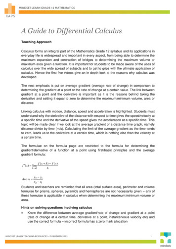
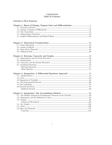
Example 1.2. Is P (5,12) on the line joining Q(2,7) and R(8,15)?The slope of the line through Q and R is (15 7)/(8 2) 4/3. The slope of the line through Pand Q is (12 7)/(5 2) 5/3. Since these two lines do not have the same slope, they cannot bethe same line. Thus P is not on the line through Q and R.Here are some facts about lines which will be useful when studying more general curves.a. If L is a line of slope m, then(1.6)m tan θwhere θ is the angle that L makes with a horizontal line. If the line is vertical, then L has infiniteslope.Suppose we are given two lines: L1 of slope m1 , and L2 of slope m2 . Thenb. L1 and L2 are parallel if and only if m1 m2 .c. L1 and L2 are perpendicular if and only if m1 m2 1.d. The length of of the line segment between two points P (x1 , y1 ) and Q(x2 , y2 ) (the distancebetween the two points) is(1.7) P Q p(x1 x2 )2 (y1 y2 )2 .Example 1.3 Find the equation of the line through (2,3) which is perpendicular to the lineL : 2x 3y 11.The line L has slope m 2/3. Thus the line perpendicular to L has slope 1/( 2/3) 3/2.Thus the equation of the line we seek isy 33 x 22or y 3x.2Polynomial functionsFor the general curve given by the equation y f (x), the ratio (1.3): y/ x is the slope of theline joining the two points (x0 , y0 ) and (x1 , y1 ) on the graph of f . But now, if the graph is not aline, this ratio changes as the point (x1 , y1 ) moves. As x1 approaches x0 , this ratio may approacha specific number. If it does, this number is called the derivative of y with respect to x, evaluatedat the point x0 . It is the instantaneous rate of change of y with respect to x at x0 , and also theslope of the line which best approximates the curve at (x0 , y0 ), called the tangent line to the curve(see Figure 1.2).3

Figure 1.2x1 y1 x1 y1 x0 y0 x1 y1 TangentLine In this chapter we shall concentrate on finding the derivative of functions given by a formula; thisprocess is called differentiation. It turns out to be quite simple for polynomial functions. But first,we make these definitions explicit.Definition 1.1. Let y f (x) be a function defined for all values of x in an interval about thepoint a. If the difference quotientf (x) f (a)x aapproaches a specific number L, then we say that f is differentiable at a, and the number L iscalled the derivative of f at a, denoted f 0 (a). It is the slope of the tangent line of y f (x) ata.For now, we will rely on an intuitive understanding of the phrase “approaches a specific numberL”; the meaning will be made clear through the examples. After these examples, we introduce anexplicit definition of the idea of limit, and in the next chapter we will discuss this definition ingreater depth.Example 1.4. Consider f (x) x2 , Find the tangent line to this curve at the point (a, f (a)).We take a point (x, f (x)) near (a, f (a)) and calculate the difference quotientf (x) f (a)x2 a2(x a)(x a) x a .)x ax ax aClearly, as x approaches a, x a approaches 2a, so we get f 0 (a) 2a.Since this is true for any value a, we can conclude that if f (x) x2 , its derivative is f 0 (x) 2x.Example 1.5. Find the equation of the line tangent to the curve y x2 at the point (3,9).For x 3, the derivative is f 0 (3) 2(3) 6. Thus the tangent line has the equationy 9 6x 3or4y 6x 9 .

The ease with which we calculated the derivative for y x2 followed from simple algebraic facts.We shall see that this works in general for polynomials; but first, one more example:Example 1.6. If f (x) x3 , f 0 (x) 3x2 . Fix a point (a, a3 ) on the graph, and let (x, x3 ) be anearby point. We look at the slope of the line joining these points:x3 a3 y . xx aSince the quotient of x3 a3 by x a is x2 ax a2 this can be rewritten asx3 a3(x a)(x2 ax a2 ) x2 ax a2 ,x ax aand evaluating this at a, we get f 0 (a) 3a2 .Now, for any polynomial y f (x), this process will work: divide f (x) f (a) by x a, and evaluatethe quotient at x a to calculate the derivative. Let’s spell this out, starting with the divisiontheorem of algebra:Theorem 1.2. Let f be a polynomial of degree d. Then, for any number a when we divide f (x)by x a, we get a quotient which is a polynomial of degree d 1 and a remainder of f (a):(1.8)f (a)f (x) q(x) .x ax aNow, to apply this to the calculation of instantaneous rate of change, move the second term onthe right to the left:f (x) f (a) q(x) .x aAas we let x approach a, the difference quotient q(x) approaches q(a), so the polynomial is differentiable at a, and its derivative is q 0 (a).Theorem 1.3. A polynomial y f (x) is everywhere differentiable. Its derivative at x a is q(a),where q is the quotient of f (x) f (a) by x a.Newton realized that using long division would be a tedious way to calculate derivatives, and withthem instantaneous rates of change, so he had the genius to take a slightly more abstract approachto lead to an automatic way of calculating derivatives. First, we must make explicit what we meanby the phrase ”the expression approaches a specific number” by introducing the notion of limit.Suppose that y g(x) defines a function in an interval about x0 . We say that g has the limit Las x approaches x0 if we can make the difference g(x) L as small as we need it to be by takingx as close to x0 as we have to. More precisely, but less intuitively,Definition 1.4. limx x0 g(x) L if, for any 0 there is a δ 0 such that x x0 δ implies g(x) L .We now observe that limits behave well under algebraic operations.5

Proposition 1.5. Suppose that f and g are functions defined in an interval about x0 and thatlim g(x) M .lim f (x) L ,x x0x x0Thenlim (f (x) g(x)) L Ma)x x0lim (f (x) · g(x)) L · Mb)x x0c) If M 6 0, thenlimx x0f (x)L .g(x)MApplying this proposition to the calculation of derivatives, we see how differentiation behaves underalgebraic operations:Proposition 1.6. Suppose that f and g are functions defined and differentiable in an interval I.Thena) f g is differentiable in I, and (f g)0 f 0 g 0 .b) f g is differentiable in I, and (f g)0 f 0 g f g 0 .We give a brief justification of these rules, which follow from the corresponding rules for limits(proposition 1.5). This is straighforward for part a), but for the product, the argument requiressome preliminary algebraic manipulation. Suppose then, that f and g are differentiable at a, andlet h f g. Then to see that h is differentiable, we must take the limit, as x approaches a off (x)g(x) f (a)g(a)h(x) h(a) .)x ax aThe product rule for limits does not apply directly, for this is not a product. However, if we addand multiply f (a)g(x), we getf (x)g(x) f (a)g(a) [(f (x) f (a))g(x)] [f (a)(g(x) g(a))] ,which leads to a sum of productsf (x)g(x) f (a)g(a)f (x) f (a)g(x) g(a) g(x) f (a).x ax ax aNow, we can take the limits using proposition 1.5. We have to note that, since g is differentiable,we also have limx a g(x) g(a).This brings us to the rule for differentiating polynomials.6

Proposition 1.7.a) If f is constant, then f 0 0.b) If f (x) axn for some positive integer n, then f 0 (x) anxn 1 .c) A polynomial is differentiated term by term, using b) for each term.To verify a), we only have to note that a constant function is unchanging; its graph is a horizontalline, so has slope 0. c) follows from the fact that the limit of a sum is the sum of the limits. b)follows by a bootstrap method. We have already seen this for n 0, 1, 2, 3. To proceed, we usethe product rule. For example, take n 4:(x4 )0 (x3 x)0 (x3 )0 x x3 x0 (3x2 )x x3 (1) 4x3 .If we have the proposition for all integers up to n 1, then we have it for n by the same method:(xn )0 (xn 1 x)0 ((n 1)xn 2 )x xn 1 (1) nxn 1 .Example 1.7. Let f (x) 2x2 3x 3. Find f 0 (x). What is the equation of the line tangent tothe curve given by y f (x), at the point (1,2)?Using proposition 1.7, we havef 0 (x) 2(2x) 3(1) 0 4x 3 .This gives the slope of the tangent line at (1,2) by evaluating at x 1 : f 0 (1) 4(1) 3 1.Thus the equation of the tangent line isy 2 1 orx 1y x 1Example 1.8. Iff (x) 2x5 x4 8x3 2x 5 ,thenf 0 (x) 2(5x4 ) 4x3 8(3x2 ) 2x0 0 10x4 4x3 24x2 2 .If a function f is differentiable at every point of an interval I, then the derivative is defined atevery point in the interval I, and thus is a function on I. This function, denoted f 0 , is defined bythe rule: for all x in I,(1.9)f (x h) f

1.5. Implicit Differentiation and Related Rates 19 Chapter 2. Theoretical Considerations 24 2.1. Limit Operations 24 2.2. Limits at Infinity 29 2.3. Some Basic Theorems 34 2.4. l'Hopitals Rule 36 Chapter 3. Extrema, Concavity and Graphs 40 3.1. Monotonicity and the First Derivative 40 3.2. Optimization 42 3.3. Concavity and the Second .