Transcription
Mathematical Foundations of Computer NetworkingbyS. Keshav
To Nicole, my foundation
IntroductionMotivationGraduate students, researchers, and practitioners in the field of computer networking often require a firm conceptual understanding of one or more of its theoretical foundations. Knowledge of optimization, information theory, game theory, controltheory, and queueing theory is assumed by research papers in the field. Yet these subjects are not taught in a typical computerscience undergraduate curriculum. This leaves only two alternatives: either to study these topics on one’s own from standardtexts or take a remedial course. Neither alternative is attractive. Standard texts pay little attention to computer networking intheir choice of problem areas, making it a challenge to map from the text to the problem at hand. And it is inefficient torequire students to take an entire course when all that is needed is an introduction to the topic.This book addresses these problems by providing a single source to learn about the mathematical foundations of computernetworking. Assuming only a rudimentary grasp of calculus, it provides an intuitive yet rigorous introduction to a wide rangeof mathematical topics. The topics are covered in sufficient detail so that the book will usually serve as both the first and ultimate reference. Note that the topics are selected to be complementary to those found in a typical undergraduate computer science curriculum. The book, therefore, does not cover network foundations such as discrete mathematics, combinatorics, orgraph theory.Each concept in the book is described in four ways: intuitively; using precise mathematical notation; with a carefully chosennumerical example; and with a numerical exercise to be done by the reader. This progression is designed to gradually deepenunderstanding. Nevertheless, the depth of coverage provided here is not a substitute for that found in standard textbooks.Rather, I hope to provide enough intuition to allow a student to grasp the essence of a research paper that uses these theoretical foundations.OrganizationThe chapters in this book fall into two broad categories: foundations and theories. The first five foundational chapters coverprobability, statistics, linear algebra, optimization, and signals, systems and transforms. These chapters provide the basis forthe four theories covered in the latter half of the book: queueing theory, game theory, control theory, and information theory.Each chapter is written to be as self-contained as possible. Nevertheless, some dependencies do exist, as shown in Figure 1,where light arrows show weak dependencies and bold arrows show strong dependencies.Signals, Systemsand TransformsLinear algebraControl theoryGame theoryOptimizationProbabilityQueueing theoryStatisticsInformation theory
FIGURE 1.Chapter organizationUsing this bookThe material in this book can be completely covered in a sequence of two graduate courses, with the first course focussing onthe first five chapters and the second course on the latter four. For a single-semester course, some posible alternatives are tocover: probability, statistics, queueing theory, and information theorylinear algebra, signals, systems and transforms, control theory and game theorylinear algebra, signals, systems and transforms, control theory, selected portions of probability, and information theorylinear algebra, optimization, probability, queueing theory, and information theoryThis book is designed for self-study. Each chapter has numerous solved examples and exercises to reinfornce concepts. Myaim is to ensure that every topic in the book should be accessible to the perservering reader.AcknowledgementsI have benefitted immensely from the comments of dedicated reviewers on drafts of this book. Two in particular who standout are Alan Kaplan, whose careful and copious comments improved every aspect of the book, and Prof. Johnny Wong, whonot only reviewed multiple drafts of the chapters on probability on statistics, but also used a draft to teach two graduatecourses at the University of Waterloo.I would also like to acknowledge the support I received from experts who reviewed individual chapters: AugustinChaintreau, Columbia (probability and queueing theory), Tom Coleman, Waterloo (optimization), George Labahn, Waterloo(linear algebra), Kate Larson, Waterloo (game theory), Abraham Matta, Boston University (statistics, signals, systems, transforms, and control theory), Sriram Narasimhan, Waterloo (control theory), and David Tse, UC Berkeley (information theory).I received many corrections from my students at the University of Waterloo who took two courses based on book drafts inFall 2008 and Fall 2011. These are: Andrew Arnold, Nasser Barjesteh, Omar Beg, Abhirup Chakraborty, Betty Chang, LeilaChenaei, Francisco Claude, Andy Curtis, Hossein Falaki, Leong Fong, Bo Hu, Tian Jiang, Milad Khalki, Robin Kothari,Alexander Laplante, Constantine Murenin, Earl Oliver, Sukanta Pramanik, Ali Rajabi, Aaditeshwar Seth, Jakub Schmidtke,Kanwaljit Singh, Kellen Steffen, Chan Tang, Alan Tsang, Navid Vafei, and Yuke Yang.Last but not the least, I would never have completed this book were it not for the unstinting support and encouragement fromevery member of my family for the last four years. Thank you.S. KeshavWaterloo, October 2011.
CHAPTER 1Probability 1Introduction1Outcomes 1Events 2Disjunctions and conjunctions of eventsAxioms of probability 3Subjective and objective probability 4Joint and conditional probability25Joint probability 5Conditional probability 5Bayes’ rule 8Random variables10Distribution 11Cumulative density function 12Generating values from an arbitrary distribution 13Expectation of a random variable 13Variance of a random variable 15Moments and moment generating functions15Moments 16Moment generating functions 16Properties of moment generating functions 17Standard discrete distributions 18Bernoulli distribution 18Binomial distribution 18Geometric distribution 20Poisson distribution 20Standard continuous distributions 21Uniform distribution 21Gaussian or Normal distribution 21Exponential distribution 23Power law distribution 25Useful theorems 26Markov’s inequality 26Chebyshev’s inequality 27Chernoff bound 28Strong law of large numbers 29Central limit theorem 30Jointly distributed random variables31Bayesian networks 33Further ReadingExercisesCHAPTER 23535Statistics 39Sampling a population39Types of sampling 40Scales 41Outliers 41Describing a sample parsimoniously41Tables 42Bar graphs, histograms, and cumulative histograms 42The sample mean 43The sample median 46
Measures of variability 46Inferring population parameters from sample parameters 48Testing hypotheses about outcomes of experiments 51Hypothesis testing 51Errors in hypothesis testing 51Formulating a hypothesis 52Comparing an outcome with a fixed quantity 53Comparing outcomes from two experiments 54Testing hypotheses regarding quantities measured on ordinal scalesFitting a distribution 58Power 60Independence and dependence: regression, and correlation5661Independence 61Regression 62Correlation 64Comparing multiple outcomes simultaneously: analysis of varianceOne-way layout 68Multi-way layouts 70Design of experiments70Dealing with large data sets 71Common mistakes in statistical analysis 72What is the population? 72Lack of confidence intervals in comparing results 72Not stating the null hypothesis 73Too small a sample 73Too large a sample 73Not controlling all variables when collecting observations 73Converting ordinal to interval scales 73Ignoring outliers 73Further readingExercisesCHAPTER 37374Linear AlgebraVectors and matrices7777Vector and matrix algebra78Addition 78Transpose 78Multiplication 79Square matrices 80Exponentiation 80Matrix exponential 80Linear combinations, independence, basis, and dimensionLinear combinations 80Linear independence 81Vector spaces, basis, and dimension 82Solving linear equations using matrix algebra82Representation 82Elementary row operations and Gaussian elimination 83Rank 84Determinants 85Cramer’s theorem 86The inverse of a matrix 87Linear transformations, eigenvalues and eigenvectors888067
A matrix as a linear transformation 88The eigenvalue of a matrix 89Computing the eigenvalues of a matrix 91Why are eigenvalues important? 93The role of the principal eigenvalue 94Finding eigenvalues and eigenvectors 95Similarity and diagonalization 96Stochastic matrices98Computing state transitions using a stochastic matrix 98Eigenvalues of a stochastic matrix 99ExercisesCHAPTER 4101Optimization 103System modelling and optimization103An introduction to optimization 105Optimizing linear systems107Network flow 109Integer linear programming110Total unimodularity 112Weighted bipartite matching 112Dynamic programming113Nonlinear constrained optimization114Lagrangian techniques 115Karush-Kuhn-Tucker conditions for nonlinear optimization 116Heuristic non-linear optimization117Hill climbing 117Genetic algorithms 118ExercisesCHAPTER 5118Signals, Systems, and Transforms 121Introduction121Background121Sinusoids 121Complex numbers 123Euler’s formula 123Discrete-time convolution and the impulse function 126Continuous-time convolution and the Dirac delta function 128Signals130The complex exponential signal 131Systems132Types of systems133Analysis of a linear time-invariant system134The effect of an LTI system on a complex exponential inputThe output of an LTI system with a zero input 135The output of an LTI system for an arbitrary input 137Stability of an LTI system 137Transforms138The Fourier series139The Fourier Transform142Properties of the Fourier transform 144134
The Laplace Transform148Poles, Zeroes, and the Region of convergence 149Properties of the Laplace transform 150The Discrete Fourier Transform and Fast Fourier Transform153The impulse train 153The discrete-time Fourier transform 154Aliasing 155The Discrete-Time-and-Frequency Fourier Transform and the Fast Fourier Transform (FFT) 157The Fast Fourier Transform 159The Z Transform161Relationship between Z and Laplace transform 163Properties of the Z transform 164Further ReadingExercisesCHAPTER 6166166Stochastic Processes and Queueing Theory 169Overview169A general queueing system 170Little’s theorem 170Stochastic processes171Discrete and continuous stochastic processes 172Markov processes 173Homogeneity, state transition diagrams, and the Chapman-Kolmogorov equations 174Irreducibility 175Recurrence 175Periodicity 176Ergodicity 176A fundamental theorem 177Stationary (equilibrium) probability of a Markov chain 177A second fundamental theorem 178Mean residence time in a state 179Continuous-time Markov Chains179Markov property for continuous-time stochastic processes 179Residence time in a continuous-time Markov chain 180Stationary probability distribution for a continuous-time Markov chainBirth-Death processes 181Time-evolution of a birth-death process 181Stationary probability distribution of a birth-death process 182Finding the transition-rate matrix 182A pure-birth (Poisson) process 184Stationary probability distribution for a birth-death process 185The M/M/1 queue186Two variations on the M/M/1 queue189The M/M/ queue: a responsive server 189M/M/1/K: bounded buffers 190Other queueing systems192M/D/1: deterministic service times 192G/G/1 193Networks of queues 193Further readingExercises194194180
CHAPTER 7Game Theory197Concepts and terminology197Preferences and preference ordering 197Terminology 199Strategies 200Normal- and extensive-form games 201Response and best response 203Dominant and dominated strategy 203Bayesian games 204Repeated games 205Solving a game205Solution concept and equilibrium 205Dominant strategy equilibria 206Iterated removal of dominated strategies 207Maximin equilibrium 207Nash equilibria 209Correlated equilibria 211Other solution concepts 212Mechanism design212Examples of practical mechanisms 212Three negative results 213Two examples 214Formalization 215Desirable properties of a mechanism 216Revelation principle 217Vickrey-Clarke-Groves mechanism 217Problems with VCG mechanisms 219Limitations of game theoryFurther ReadingExercisesCHAPTER 8220221221Elements of Control Theory 223Introduction223Overview of a Controlled SystemModelling a System223225Modelling approach 226Mathematical representation 226A First-order System230A Second-order System231Case 1: - an undamped system 231Case 2: - an underdamped system 232Critically damped system () 233Overdamped system () 234Basics of Feedback Control235System goal 236Constraints 237PID Control238Proportional mode control 239Integral mode control 240Derivative mode control 240Combining modes 241Advanced Control Concepts241
Cascade control 242Control delay 242Stability245BIBO Stability Analysis of a Linear Time-invariant System 246Zero-input Stability Analysis of a SISO Linear Time-invariant SystemPlacing System Roots 249Lyapunov stability 250State-space Based Modelling and Control251State-space based analysis 251Observability and Controllability 252Controller design 253Digital control254Partial fraction expansion 255Distinct roots 256Complex conjugate roots 256Repeated roots 257Further readingExercisesCHAPTER 9258258Information TheoryIntroduction261261A Mathematical Model for CommunicationFrom Messages to SymbolsSource Coding261264265The Capacity of a Communication Channel270Modelling a Message Source 271The Capacity of a Noiseless Channel 272A Noisy Channel 272The Gaussian Channel278Modelling a Continuous Message Source 278A Gaussian Channel 280The Capacity of a Gaussian Channel 281Further ReadingExercises284284Solutions to Exercises 287ProbabilityStatistics287290Linear AlgebraOptimization293296Transform domain techniquesQueueing theoryGame theory304307Control Theory 309Information Theory312300249
DRAFT - Version 3 -OutcomesCHAPTER 1Probability1.1 IntroductionThe concept of probability pervades every aspect of our life. Weather forecasts are couched in probabilistic terms, as are economic predictions and even outcomes of our own personal decisions. Designers and operators of computer networks need tooften think probabilistically, for instance, when anticipating future traffic workloads or computing cache hit rates. From amathematical standpoint, a good grasp of probability is a necessary foundation to understanding statistics, game theory, andinformation theory. For these reasons, the first step in our excursion into the mathematical foundations of computer networking is to study the concepts and theorems of probability.This chapter is a self-contained introduction to the theory of probability. We begin by introducing the elementary concepts ofoutcomes, events, and sample spaces, which allows us to precisely define the conjunctions and disjunctions of events. Wethen discuss concepts of conditional probability and Bayes’ rule. This is followed by a description of discrete and continuousrandom variables, expectations and other moments of a random variable, and the Moment Generating Function. We discusssome standard discrete and continuous distributions and conclude with some useful theorems of probability and a descriptionof Bayesian networks.Note that in this chapter, as in the rest of the book, the solved examples are an essential part of the text. They provide a concrete grounding for otherwise abstract concepts and are necessary to understand the material that follows.1.1.1OutcomesThe mathematical theory of probability uses terms such as ‘outcome’ and ‘event’ with meanings that differ from those incommon practice. Therefore, we first introduce a standard set of terms to precisely discuss probabilistic processes. Theseterms are shown in bold font below. We will use the same convention to introduce other mathematical terms in the rest of thebook.Probability measures the degree of uncertainty about the potential outcomes of a process. Given a set of distinct and mutually exclusive outcomes of a process, denoted { o 1, o 2, } , called the sample space S, the probability of any outcome,denoted P(oi), is a real number between 0 and 1, where 1 means that the outcome will surely occur, 0 means that it surely willnot occur, and intermediate values reflect the degree to which one is confident that the outcome will or will not occur1. Weassume that it is certain that some element in S occurs. Hence, the elements of S describe all possible outcomes and the sumof probability of all the elements of S is always 1.1. Strictly speaking, S must be a measurable σ field.1
DRAFT - Version 3 - IntroductionEXAMPLE 1: SAMPLE SPACE AND OUTCOMESImagine rolling a six-faced die numbered 1 through 6. The process is that of rolling a die and an outcome is the numbershown on the upper horizontal face when the die comes to rest. Note that the outcomes are distinct and mutually exclusivebecause there can be only one upper horizontal face corresponding to each throw.The sample space is S {1, 2, 3, 4, 5, 6} which has a size S 6 . If the die is fair, each outcome is equally likely and the1 1probability of each outcome is ----- --- .S 6 EXAMPLE 2: INFINITE SAMPLE SPACE AND ZERO PROBABILITYImagine throwing a dart at random on to a dartboard of unit radius. The process is that of throwing a dart and the outcome isthe point where the dart penetrates the dartboard. We will assume that this is point is vanishingly small, so that it can bethought of as a point on a two-dimensional real plane. Then, the outcomes are distinct and mutually exclusive.The sample space S is the infinite set of points that lie within a unit circle in the real plane. If the dart is thrown truly randomly, every outcome is equally likely; because there are an infinity of outcomes, every outcome has a probability of zero.We need special care in dealing with such outcomes. It turns out that, in some cases, it is necessary to interpret the probability of the occurrence of such an event as being vanishingly small rather than exactly zero. We consider this situation ingreater detail in Section 1.1.5 on page 4. Note that although the probability of any particular outcome is zero, the probabilityaassociated with any subset of the unit circle with area a is given by --- , which tends to zero as a tends to zero.π 1.1.2EventsThe definition of probability naturally extends to any subset of elements of S, which we call an event, denoted E. If the sample space is discrete, then every event E is an element of the power set of S, which is the set of all possible subsets of S. Theprobability associated with an event, denoted P ( E ) , is a real number 0 P ( E ) 1 and is the sum of the probabilities associated with the outcomes in the event.EXAMPLE 3: EVENTSContinuing with Example 1, we can define the event “the roll of a die results in a odd-numbered outcome.” This corresponds1 1 11to the set of outcomes {1,3,5}, which has a probability of --- --- --- --- . We write P({1,3,5}) 0.5.6 6 62 1.1.3Disjunctions and conjunctions of eventsConsider an event E that is considered to have occurred if either or both of two other events E 1 or E 2 occur, where bothevents are defined in the same sample space. Then, E is said to be the disjunction or logical OR of the two events denotedE E 1 E 2 and read “ E 1 or E 2 .”EXAMPLE 4: DISJUNCTION OF EVENTS2
DRAFT - Version 3 -Axioms of probabilityContinuing with Example 1, we define the events E 1 “the roll of a die results in an odd-numbered outcome” and E 2 “the roll of a die results in an outcome numbered less than 3.” Then, E 1 { 1, 3, 5 } and E 2 { 1, 2 } andE E 1 E 2 { 1, 2, 3, 5 } . In contrast, consider event E that is considered to have occurred only if both of two other events E 1 or E 2 occur, where bothare in the same sample space. Then, E is said to be the conjunction or logical AND of the two events denoted E E 1 E 2and read “ E 1 and E 2 .”. When the context is clear, we abbreviate this to E E 1 E 2 .EXAMPLE 5: CONJUNCTION OF EVENTSContinuing with Example 4, E E 1 E 2 E 1 E 2 { 1 } . Two events Ei and Ej in S are mutually exclusive if only one of the two may occur simultaneously. Because the events haveno outcomes in common, P ( E i E j ) P ( { } ) 0. Note that outcomes are always mutually exclusive but events need notbe so.1.1.4Axioms of probabilityOne of the breakthroughs in modern mathematics was the realization that the theory of probability can be derived from just ahandful of intuitively obvious axioms. Several variants of the axioms of probability are known. We present the axioms asstated by Kolmogorov to emphasize the simplicity and elegance that lie at the heart of probability theory:1.0 P ( E ) 1 , that is, the probability of an event lies between 0 and 1.2.P(S) 1, that is, it is certain that at least some event in S will occur.3.Given a potentially infinite set of mutually exclusive events E1, E2,. P E i P ( E i ) i 1 i 1(EQ 1)That is, the probability that any one of the events in the set of mutually exclusive events occurs is the sum of their individual probabilities. For any finite set of n mutually exclusive events, we can state the axiom equivalently as:n n P Ei P ( Ei ) i 1 i 1(EQ 2)P ( E1 E2 ) P ( E1 ) P ( E2 ) – P ( E1 E2 )(EQ 3)An alternative form of Axiom 3 is:This alternative form applies to non-mutually exclusive events.EXAMPLE 6: PROBABILITY OF UNION OF MUTUALLY EXCLUSIVE EVENTSContinuing with Example 1, we define the mutually exclusive events {1,2} and {3,4} which both have a probability of 1/3.1 12Then, P ( { 1, 2 } { 3, 4 } ) P ( { 1, 2 } ) P ( { 3, 4 } ) --- --- --- .3 333
DRAFT - Version 3 - Introduction EXAMPLE 7: PROBABILITY OF UNION OF NON-MUTUALLY EXCLUSIVE EVENTSContinuing with Example 1, we define the non-mutually exclusive events {1,2} and {2,3} which both have a probability of1 12 111/3. Then, P ( { 1, 2 } { 2, 3 } ) P ( { 1, 2 } ) P ( { 2, 3 } ) – P ( { 1, 2 } { 2, 3 } ) --- --- – P ( { 2 } ) --- – --- --- .3 33 62 1.1.5Subjective and objective probabilityThe axiomatic approach is indifferent as to how the probability of an event is determined. It turns out that there are two distinct ways in which to determine the probability of an event. In some cases, the probability of an event can be derived fromcounting arguments. For instance, given the roll of a fair die, we know that there are only six possible outcomes, and that alloutcomes are equally likely, so that the probability of rolling, say, a 1, is 1/6. This is called its objective probability. Anotherway of computing objective probabilities is to define the probability of an event as being the limit of a counting process, asthe next example shows.EXAMPLE 8: PROBABILITY AS A LIMITConsider a measurement device that measures the packet header types of every packet that crosses a link. Suppose that during the course of a day the device samples 1,000,000 packets and of these 450,000 packets are UDP packets, 500,000 packetsare TCP packets, and the rest are from other transport protocols. Given the large number of underlying observations, to a firstapproximation, we can consider that the probability that a randomly selected packet uses the UDP protocol to be 450,000/Lim1,000,000 0.45. More precisely, we state: P ( UDP ) ( UDPCount ( t ) ) ( TotalPacketCoun ( t ) )t where UDPCount(t) is the number of UDP packets seen during a measurement interval of duration t, and TotalPacketCount(t) is the total number of packets seen during the same measurement interval. Similarly P(TCP) 0.5.Note that in reality the mathematical limit cannot be achieved because no packet trace is infinite. Worse, over the course of aweek or a month the underlying workload could change, so that the limit may not even exist. Therefore, in practice, we areforced to choose ‘sufficiently large’ packet counts and hope that the ratio thus computed corresponds to a probability. Thisapproach is also called the frequentist approach to probability. In contrast to an objective assessment of probability, we can also use probabilities to characterize events subjectively.EXAMPLE 9: SUBJECTIVE PROBABILITY AND ITS MEASUREMENTConsider a horse race where a favoured horse is likely to win, but this is by no means assured. We can associate a subjectiveprobability with the event, say 0.8. Similarly, a doctor may look at a patient’s symptoms and associate them with a 0.25 probability of a particular disease. Intuitively, this measures the degree of confidence that an event will occur, based on expertknowledge of the situation that is not (or cannot be) formally stated.How is subjective probability to be determined? A common approach is to measure the odds that a knowledgeable personwould bet on that event. Continuing with the example, if a bettor really thought that the favourite would win with a probability of 0.8, then the bettor should be willing to bet 1 under the terms: if the horse wins, the bettor gets 1.25, and if the horseloses, the bettor gets 0. With this bet, the bettor expects to not lose money, and if the reward is greater than 1.25, the bettorwill expect to make money. So, we can elicit the implicit subjective probability by offering a high reward, and then loweringit until the bettor is just about to walk away, which would be at the 1.25 mark. 4
DRAFT - Version 3 -Joint probabilityThe subjective and frequentist approaches interpret zero-probability events differently. Consider an infinite sequence of successive events. Any event that occurs only a finite number of times in this infinite sequence will have a frequency that can bemade arbitrarily small. In number theory, we do not and cannot differentiate between a number that can be made arbitrarilysmall and zero. So, from this perspective, such an event can be considered to have a probability of occurrence of zero eventhough it may occur a finite number of times in the sequence.From a subjective perspective, a zero-probability event is defined as an event E such that a rational person would be willingto bet an arbitrarily large but finite amount that E will not occur. More concretely, suppose this person were to receive areward of 1 if E did not occur but would have to forfeit a sum of F if E occurred. Then, the bet would be taken for anyfinite value of F.1.2 Joint and conditional probabilityThus far, we have defined the terms used in studying probability and considered single events in isolation. Having set thisfoundation, we now turn our attention to the interesting issues that arise when studying sequences of events. In doing so, itis very important to keep track of the sample space in which the events are defined: a common mistake is to ignore the factthat two events in a sequence may be defined on different sample spaces.1.2.1Joint probabilityConsider two processes with sample spaces S 1 and S 2 that occur one after the other. The two processes can be viewed as asingle joint process whose outcomes are the tuples chosen from the product space S 1 S 2 . We refer to the subsets of theproduct space as joint events. Just as before, we can associate probabilities with outcomes and events in the product space.To keep things straight, in this section, we denote the sample space associated with a probability as a subscript, so thatP S ( E ) denotes the probability of event E defined over sample space S 1 and P S S ( E ) is an event defined over the prod112uct space S 1 S 2 .EXAMPLE 10: JOINT PROCESS AND JOINT EVENTSConsider sample space S 1 { 1, 2, 3 } and sample space S 2 { a, b, c } . Then, the product space is given by{ ( 1, a ), ( 1, b ), ( 1, c ), ( 2, a ), ( 2, b ), ( 2, c ), ( 3, a ), ( 3, b ), ( 3, c ) } . If these events are equiprobable, then the probability of1each tuple is --- . Let E { 1, 2 } be an event in S 1 and F { b } be an event in S 2 . Then the event EF is given by the91 12tuples {(1, b), (2, b)} and has probability --- --- --- .9 99 We will return to the topic of joint processes in Section 1.8 on page 31. We now turn our attention to the concept of conditional probability.1.2.2Conditional probabilityCommon experience tells us that if a sky is sunny, there is no chance of rain in the immediate future, but that if it is cloudy, itmay or may not rain soon. Knowing that the sky is cloudy, therefore, increases the chance that it may rain soon, compared tothe situation when it is sunny. How can we formalize this intuition?5
DRAFT - Version 3 - Joint and conditional probabilityTo keep things simple, first consider the case when two events E and F share a common sample space S and occur one afterthe other. Suppose that the probability of E is P S ( E ) and the probability of F is P S ( F ) . Now, suppose that we are informedthat event E actually occurred. By definition, the conditional probability of the event F conditioned on the occurrence ofevent E is denoted P S S ( F E ) (read “the probability of F given E”) and computed as:PS S ( E F )P S S ( EF )P S S ( F E ) ------------------------------- ------------------------PS ( E )PS( E )(EQ 4)If knowing that E occurred does not affect the probability of F, E and F are said to be independent andP S S ( EF ) P S ( E )P S ( F )EXAMPLE 11: CONDITIONAL PROBABILITY OF EVENTS DRAWN FROM THE SAME SAMPLE SPACEConsider sample space S { 1, 2, 3 } and events E { 1 } and F { 3 } . Let P S ( E ) 0.5 and P S ( F ) 0.25 . Clearly,the space S S { ( 1, 1 ), ( 1, 2 ), , ( 3, 2 ), ( 3, 3 ) } . The joint event EF { ( 1, 3 ) } . Suppose P S S ( EF ) 0.3 . Then,P S S ( EF )P S S ( F E ) ------------------------- 0.3------- 0.6 . We interpret this to mean that if event E occurred, then the probability that event0.5PS ( E )F occurs is 0.6. This is higher than the probability of F occurring on its own (which is 0.25). Hence, the fact the E occurredimproves the chances of F occurring, so the two events are not independe
Graduate students, researchers, and practitioners in the field of computer networking often require a firm conceptual under-standing of one or more of its theoretical foundations. Knowledge of optimization, information theory, game theory, control theory, and queueing theory is assumed by re search papers in the field.