Transcription
Credit: 2 PDHCourse Title:Soil-Structure InteractionApproved for Credit in All 50 StatesVisit epdhonline.com for state specific informationincluding Ohio’s required timing feature.3 Easy Steps to Complete the Course:1. Read the Course PDF2. Purchase the Course Online & Take the Final Exam3. Print Your Certificateepdh.com is a division of Cer fied Training Ins tute
Chapter 6Soil-Structure InteractionAlexander TyapinAdditional information is available at the end of the chapterhttp://dx.doi.org/10.5772/483331. IntroductionFirst the very definition of the soil-structure interaction (SSI) effects is discussed, because itis somewhat peculiar: every seismic structural response is caused by soil-structureinteraction forces, but only in certain situations they talk about soil-structure interaction(SSI) effects. Then a brief history of this research field is given covering the last 70 years.Basic superposition of wave fields is discussed as a common basis for different approaches –direct and impedance ones, first of all. Then both approaches are described and applied to asimple 1D SSI problem enabling the exact solution. Special attention is paid to the substitutionof the boundary conditions in the direct approach often used in practice. Impedance behavioris discussed separately with principal differentiation of quasi-homogeneous sites and siteswith bedrock. Locking and unlocking of layered sites is discussed as one of the main waveeffects. Practical tools to deal with SSI are briefly described, namely LUSH, SASSI and CLASSI.Combined asymptotic method (CAM) is presented.Nowadays SSI models are linear. Nonlinearity of the soil and soil-structure contact is treatedin a quasi-linear way. Special approach used in SHAKE code is discussed and illustrated.Some non-mandatory additional assumptions (rigidity of the base mat, horizontal layeringof the soil, vertical propagation of seismic waves) often used in SSI, are discussed. Finally,two of the SSI effects are shown on a real world example of the NPP building. The first effectis soil flexibility; the second effect is embedment of the base mat. Recommendations toengineers are summed in conclusions.2. Peculiarities of the SSI definitionSoil-structure interaction (SSI) analysis is a special field of earthquake engineering. It isworth starting with definition. Common sense tells us that every seismic structural responseis caused by soil-structure interaction forces impacting structure (by the definition of seismicexcitation). However, engineering community used to talk about soil-structure interaction 2012 Tyapin, licensee InTech. This is an open access chapter distributed under the terms of the CreativeCommons Attribution License (http://creativecommons.org/licenses/by/3.0), which permits unrestricted use,distribution, and reproduction in any medium, provided the original work is properly cited.
146 Earthquake Engineeringonly when these interaction forces are able to change the basement motion as compared tothe free-field ground motion (i.e. motion recorded on the free surface of the soil withoutstructure). So, historically the conventional definition of SSI is different from simpleoccurrence of the interaction forces: these forces occur for every structure, but not alwaysthey are able to change the soil motion.This simple fact leads to the important consequences. If a structure can be analyzed as basedon rigid foundation with free-field motion at it, then they use to say that “no SSI effectsoccur” (though structure is in fact moved by the interaction forces, and the same forcesimpact the foundation). Looking at the variety of the real-world situations, we can concludethat only part of them satisfies the conventional definition of SSI.The ability of the interaction forces to change the soil motion depends, of course, on twofactors: value of the force and flexibility of the soil foundation. The value of the interactionforce may be often estimated via the base mat acceleration and inertia of the structure. Forgiven soil site and given free-field seismic excitation the heavier is the structure, the morelikely SSI effects occur. Usually most of civil structures resting on hard or medium soils donot show the signs of considerable SSI effects.From the inertial point of view, the heaviest structures we deal with are hydro-structures(like dams) and nuclear power plant (NPP) main structures – first of all, reactor buildings.So, the development of the SSI field in the earthquake engineering was historically linked tothe development of these two fields of industry.From the soil flexibility point of view, for the given structure and given free-field seismicexcitation the softer is the soil, the more likely SSI effects occur. Soil shear module is aproduct of mass density and square of the shear wave velocity. Mass density of soil inpractice varies around 2,0 t/m3 in a comparatively narrow range, so the main characteristicof the soil stiffness is shear wave velocity Vs. Usually soil is considered “soft” when Vs is lessthan 300 m/s, and “hard” when Vs is greater than 800 m/s. If Vs is greater than 1100 m/s, theyusually talk about “rigid” soil (no SSI effects – just rigid platform with a structure on it andexcitation taken from the free field).All these ranges are of course purely empirical. Obviously, one and the same soil can behaveas rigid one towards very light and small structure (like a tent), and behave as a soft onetowards heavy and rigid structure (like the NPP reactor building).Sometimes to decide whether to account for SSI effects they compare the natural frequenciesof the rigid structure on the flexible soil foundation with those of the flexible structure on arigid foundation. If the lowest natural frequency of the first set is greater than the firstdominant frequency of the second set two and more times, they do not consider SSI effects(e.g., see standards ASCE4-98 [1]). As SSI field is rather sophisticated, sometimes it is worthneglecting SSI, when allowed.However, one should keep in mind another situation, when SSI effects occur. In soft soilsseismic wave may have moderate wavelength comparable to the size of structure, so that
Soil-Structure Interaction 147the free-field motion over the soil-structure contact surface will have the so-called “spacevariability”. In this case a comparatively stiff structure (even a weightless one) can impactthe soil motion by structural rigidity (i.e., stiff contact soil-structure surface will not allowsoil to move in the manner it used to move without structure). So, once more the presence ofa structure changes the behavior of soil during seismic excitation, which is a SSI effect. Thisis a situation with considerably embedded structures; the same applies to the great basemats, “averaging” the travelling seismic waves [2]. But the most typical situation is a simplepile foundation – piles are used with soft soils, they are not rigid but usually stiff enough tochange the foundation motion.To conclude this part, let us talk a little about the so-called SSSI – structure-soil-structureinteraction. When a group of structures is resting on a common soil foundation, the basemat motion of a structure may be changed (as compared to the free-filed motion) notbecause of this very structure only, but because of the neighboring structures. Of course, ifall structures are comparatively light and no SSI effects occur for each of them standingalone, usually no SSSI effects occur for the group. But in case at least one of the structuresstanding alone can cause SSI effects, the additional waves in the soil (i.e. additional to thefree-field wave picture) will spread from this structure, impacting neighbors. Sometimes (forthe light/small neighbors) this situation can be analyzed without SSI but with special seismicexcitation, accounting for the influence of the heavy neighbor. In other cases severalstructures should be analyzed together because of the mutual influence.Thus, general goal of the SSI analysis is to calculate seismic response of structure based onseismic response of free field (sometimes free field may differ from the final soil). Generalformat of the SSI analyses results is basements’ motion obtained using the information abouta) soil foundation (sometimes the initial one and the final one separately), b) structure, c)seismic excitation provided without structures. Another format of the SSI results is soilstructure interaction forces, necessary to estimate the soil foundation capability to withstandearthquake. Sometimes, the complete structural seismic response is obtained together withSSI in the format of response motion of different structural nodes and response structuralinternal seismic forces.3. Brief historyAs SSI field combines structures’ and soil modeling, the level of such modeling is generallylower than in the classical soil mechanics and in the structural mechanics standing alone.For several decades (up to 1960-s) only soil flexibility was considered without soil inertia –springs modeled soil. At that time mostly the machinery basements were analyzed for thedynamic interaction with soil foundation (the largest of them probably being turbines). Infact, it was a quasi-static approach – the well-known static solution for rigid stamps, beamsand plates on elastic foundation was applied at every time step. The model was so simple,that nobody even used the special term “SSI” at that time. The key question of such a simpleapproach appeared to be damping. The material damping measured in the laboratories with
148 Earthquake Engineeringsoil samples proved to be considerably less than the damping measured in the dynamicfield tests with rigid stamps resting on the soil surface.The nature of this effect was discovered in 1930-40s (Reissner in Germany [3], Schechter inthe USSR) and proved to be in inertial properties of the soil. Inertia plus flexibility alwaysmean wave propagation. It turned out that in the field tests actual energy dissipation in thesoil was composed of two parts: conventional “material” damping (the same as inlaboratory tests) and so-called “wave damping”. In the latter case the moving stamp causedcertain waves in the soil, and those waves took away energy from the stamp, contributing tothe overall “damping” in the soil-structure system. This energy was not transferred frommechanical form into heat (like in material damping case), but was taken to the infinity inthe original mechanical form. In reality waves did not go to the infinity, graduallydissipating due to the material damping in the soil, but huge volumes of the soil wereinvolved in this wave propagation. Even without any material damping in the soil this“wave damping” contributed a lot to the response of the stamp. In practice it turned out thatthe level of wave damping was usually greater than the level of material damping.In parallel it turned out that when the base mat size is comparable to the wave length in thesoil, not only damping, but stiffness also depends on the excitation frequency. This effect isinvisible for comparatively small machine basements, but important for large and stiffstructures.To study these wave effects new soil-structure models with infinite inertial soil foundationsshould be considered. That was the moment (1960-s) when the very term “SSI” appeared[2,4,5]. It happened so, that NPPs were actively designed at that time, including seismicregions (e.g., California), and intensive research was funded in the US to study the SSIeffects controlling the NPP seismic response. Earthquake Engineering Research Center(EERC) in the University of Berkley, California became a leader with such outstandingscientists as H.B.Seed and J.Lysmer on board [6].The main result of these investigations was the development of new powerful tools toanalyze more or less realistic models. The earlier SSI models considered homogeneous halfspace with surface rigid stamp. They could be treated analytically or semi-analytically forsimple stamp shapes (e.g., circle).In practice soil is usually layered. Layering can lead to the appearance of the new wavetypes and change the whole wave picture. Important achievements of 1960-70s enabled tomove from the homogeneous half-space to the horizontally–layered medium in soilmodeling [7,8]. However, the infinite part of the foundation, excluding some limited soilvolume around the basement, still remains a) linear, b) isotropic, c) horizontally layered.These limitations are due to the methods of the SSI analysis. The final masterpiece of Prof.Lysmer was SASSI code [9], further developed by F.Ostadan, M.Tabatabaie, D.Giocel et al.This code combined finite element modeling of the structure and limited volume of the soilwith semi-analytical modeling of the infinite foundation (see below). Limitations on theembedment depth and on the shape of the underground part have gone.
Soil-Structure Interaction 149Some other scientists have greatly contributed to this field approximately at the same time(J.Wolf [10,11], J.M.Roesset, E.Kausel [12] and J.Luco [4] should be mentioned).After the Three Miles Island and Chernobyl accidents there was a long pause in the nuclearenergy development in the West (e.g., in 2012 US NRC issued a first permission for a newNPP block in last 33 years) and in Russia (due to the economic problems of 1990s), though inAsia they continued to build new blocks. SSI investigations went forward in South Korea,China, India. Nowadays, in spite of the Fukushima accident, nuclear industry goes forward.In parallel SSI was studied by hydro-engineers (for the dams design, first of all). However,this field separated from the “NPP field of SSI” about 40 years ago. The reason was that theSSI models usually applied in nuclear industry (horizontally layered soil, rigid or very stiffbase mats) are often not applicable to the hydro-dams situations (rocky canyons, etc.). Thatis why both models and methods used in the SSI field usually are different in nuclear andhydro-industries.In last decades, civil structures are gradually increasing in size and embedment. Effects likeSSI and SSSI from time to time are considered during the design procedures of suchstructures. Naturally, they are closer to the NPP practice than to the hydro-energy practice.The author has about 30 years of experience in nuclear industry, dealing with SSI problems.So, the subsequent text will be based on the “NPP” approach to the SSI problems.4. Basic superpositionToday there exist three approaches to SSI problems, namely “direct”, “impedance”, and“combined” ones. To understand them all, let us start from common general approach basedon the superposition of the wave fields.Let us call the problem with seismic wave, soil and structure “problem A” and start withcompletely linear soil-structure model. Let Q be some surface surrounding the basement inthe soil and dividing the soil-structure model into two parts: the “external” part Vext andinternal part Vint. Let (-F) be additional external loads distributed over Vint and speciallytuned so, to provide zero displacements in Vint. Then “problem A” can be split in the sum oftwo wave pictures: “problem A1”, including seismic excitation and loads (-F), and “problemA2” including only loads (F) without seismic wave – see Fig.1.This simple superposition leads to a number of important conclusions.1.2.3.As in “problem A1” all displacements in the internal volume Vint are zero, the motion ofVint in “problem A2” is the same as in “problem A”. Hence, if we are interested in themotion of Vint only, we can substitute “problem A” with “problem A2”.As in “problem A1” all displacements in the internal volume Vint are zero, all the strainsand internal forces in the internal volume Vint are zero, and the external loads (-F) mustbe zero everywhere in Vint, except surface Q.As in “problem A1” all displacements, strains and internal forces in the internal volumeVint are zero, no forces are impacting Q from Vint (i.e., forces impacting Q from Vext are
150 Earthquake Engineeringbalanced by loads (-F)). Hence, Vint can be withdrawn or replaced by another medium(with zero displacements) without changing Vext, seismic excitation, or loads (-F). Inparticular, Vint can be replaced by initial soil without structure.Figure 1. Basic superposition: split of the “problem A”4.5.6.We can withdraw structure from Fig.1 and call the problem with initial soil in Vint“problem B”. This problem can be also split in “problem B1” and “problem B2” in thesame manner as “problem A”. Wave fields in Vext and loads (-F) are equal in “problemA1” and “problem B1”. However, in “problem A2” and “problem B2” wave fields aredifferent in spite of similar loads F and similar Vext in both problems. Generally, themotions of Q in “problem B2” and “problem A2” are different due to the waves,radiating from the structure in “problem A2”.Wave field in volume Vint in “problem B2” is the same as in “problem B” (see conclusion 1above). Very often this field is known apriori or easily calculated. This creates a powerfultool to verify models suggested for “problem A2”. Each of these models contains somedescription of the internal part Vint, external part Vext and the loads F. It is useful to takethe same Vext and F and substitute the internal part Vint by the initial soil, thus comingfrom “problem A2” to “problem B2”. The suggested Vext and F must provide adequatesolution for “problem B2”; otherwise they cannot be applied to “problem A2”.Loads (–F) can be obtained from the wave field U0 in “problem B” and dynamicstiffness operator G0 for the initial unbounded soil as follows F( x) G0 ( x , y )[ U 0 ( y )](1)Formula (1) uses operator G0 in the time domain. This operator is applied to thedisplacement field in the volume Vint and provides the loads, distributed over the volume(this formula can be applied to the whole volume Vint, but for the internal nodes the resultwill be zero). For linear initial soil this operator in the frequency domain will turn intocomplex frequency-dependent dynamic stiffness function. Note that for the given surface Qthe loads F in (1) can be split in two parts: loads Fint acting from Vint and loads Fext actingfrom Vext. Physical meaning is illustrated in Fig.2.
Soil-Structure Interaction 151Figure 2. Split of loads F into Fint and FextWith given free-field wave field U0 one can easily obtain Fint just as surface forces at Qcorresponding to the internal stress field.Theoretically we can change the content of the volume Vint in “problem B” (e.g., withdrawthe medium completely, taking loads Fint to zero). This change will change operator G0,change wave field U0, but the left part of (1) will stay the same, as it is in fact fullydetermined by soil properties in Vext and initial seismic wave.Even if there exists some physical non-linearity in the model, and this non-linearity islocalized inside Vint, initial “problem A” can still be substituted by “problem A2” withoutchanging the loads F, as compared to the linear case. This is a consequence of the logic of theprevious point: the loads are fully determined by soil in Vext and initial seismic wave.5. Classification of methods: direct and impedance approachesCurrent methods of SSI analysis can be classified according to the choice of surface Q. In“direct” method they try to put Q on some physical boundaries in the soil, usually apartfrom the basement. In “impedance” method they put Q right on the soil-structure contactsurface, additionally presuming the rigidity of this surface. In “combined” method they putQ on the boundary of the “modified volume” (sometimes Q is a flexible soil-structurecontact surface, but sometimes there exists some additional soil volume around thebasement modified with the appearance of structure). Let us discuss some details of thesemethods one by one.5.1. Direct approachIn direct method there always exists certain volume Vint. Usually the lower boundary (i.e.,the bottom of Vint) is placed on the rock. In this case we presume that the additional wavesradiating from the structure cannot change the motion of this boundary, as compared tothe seismic field U0. As a consequence, we can substitute boundary conditions in
152 Earthquake Engineering“problem A2”, fixing the motion of the bottom (and obtaining it from “problem B”)instead of modeling Vext and applying loads F at surface Q. This substitution of theboundary conditions is shown in Fig.3.Figure 3. Substitution of the boundary conditions at the bottom of Vint in direct methodOne should remember that such substitution is accurate for rigid rock only. Otherwise, anerror occurs due to the reflection of the additional waves from such a boundary back intoVint. This error can be significant. The example will be shown below.After the lower boundary is fixed, lateral boundaries (usually vertical) remain to be set. In1970s, when direct method was popular, there was an evolution of these boundaries from“elementary” ones (fixed or free) towards more accurate ones. The first important step wasso-called “acoustic boundaries” by Lysmer and Kuhlemeyer [13,14].Physical base is as follows. 1D elastic (without material damping!) massive rod with shear orpressure waves can be cut in two, and one half of it can be accurately replaced by viscousdashpot. This is illustrated by Fig. 4.Dashpot viscosity parameter is a product of mass density ρ and wave velocity c. So, Lysmerand Kuhlemeyer suggested to place distributed “shear” and “pressure” dashpots over verticallateral boundary (three dashpots along three axes in each node). Practically they substitutedthe half-infinite layer in Fig.3 by number of horizontal 1D rods normal to the boundary.Figure 4. Analogue between half-infinite rod of unit cross-section area and viscous dashpot withviscosity parameter b ρc
Soil-Structure Interaction 153This boundary was far better than any elementary (fixed or free) boundary before.Horizontal body waves normal to the boundary did not have artificial reflection into Vint(that is why this boundary was called “non-reflecting boundary”). This boundary couldwork in the time domain. Besides, this boundary was “local”: the response force acting tothe node depended on the velocities of this node only, not neighbors.This boundary was implemented in code LUSH [15], named after the authors (Lysmer,Udaka, Seed, Hwang). However, soon it turned out that the most important waves,radiating by structure in the soil underlain by rock are not horizontal body waves, butsurface waves (see below). So, the artificial reflection at the boundary was not completelyeliminated, and such a boundary could be placed only apart from the structure (3-4 plansizes from the basements) to get more or less reasonable results.One should keep in mind the important limitation: when wave process in Vint is modeled byordinary finite elements, the element size should be about 1/8 (1/5 at most [1]) of thewavelength. It means that one cannot increase the finite element size going away from thestructure (as they often do in statics). So, the increase in Vint leads to the considerableincrease in the problem size and to the computational problems.The next step was done by G.Waas [8,16,17]. Instead of replacing the infinite soil by numberof horizontal rods he suggested to use “homogeneous solutions” – i.e. the waves in thehorizontally-layered medium underlain by rigid rock. These waves can be evaluated in thefrequency domain only. According to G.Waas, in 2D case each homogeneous displacementvaries in the horizontal direction following complex exponential rule with a certain complexfrequency-dependent “wave number”; in the vertical direction it varies according to thefinite-element interpolation. Later it turned out that in 3D case cylindrical waves in Vextalong horizontal radius followed not exponents, but certain special Hankel functions withthe same complex “wave numbers” as previously exponents in 2D case.Any displacement of the lateral boundary (in the finite-element approximation) can besplit into the sum of such waves in Vext. Then stresses are calculated at the boundary andfinally nodal forces impacting Vint from Vext in response to boundary displacement can beevaluated. So, the final format of the Waas boundary was the dynamic stiffness matrix inthe frequency domain, replacing Vext in the model. Unlike previous boundaries, thisboundary was not local: response forces from Vext in the node depended not only on themotion of this very node, but on the motion of all the nodes. Thus, dynamic stiffnessmatrix became fully populated.New boundaries (they were called “transmitting boundaries”) proved to be far moreaccurate than previous ones. They could be placed right near the basement, decreasing Vintand accelerating the analysis. So, LUSH was converted into FLUSH ( Fast LUSH) [18] for 2Dproblems. Then appeared code ALUSH ( Axisymmetric LUSH) [19] to solve 3D problemswith axisymmetric geometry. However, there remained two important limitations: hardrock at the bottom and axisymmetric geometry of structure in 3D case. The next stepforward was again done by J.Lysmer in EERC. But this new approach will be discussed later(see “combined method”).
154 Earthquake Engineering5.2. Impedance approachIf we presume the rigidity of the soil-structure contact surface and place surface Q in Fig.1right at this surface, we get six degrees of freedom for Q. Corresponding forces F in“problem A2” are condensed to six–component integral forces, loading the immovable basemat during seismic excitation. In addition, when the mat moves, Vext impacts the movingbase mat by response forces set by “dynamic stiffness matrix” 6 x 6. This matrix is a linearoperators’ matrix in the time domain for linear soil (soil in Vext was linear from the verybeginning). In the frequency domain it becomes complex frequency dependent matrix called“impedance matrix”. That is why the whole approach is called the “impedance” one.Impedances can be estimated in the field experiments with stamps excited by unbalancedrotors. They were the first parameters of the soil flexibility in the early times of SSI (whenmachinery base mats were analyzed).Let Rj(x) be real “rigid” vector displacements field of the contact surface Q, when one of sixgeneral coordinates of the surface Q (coordinate number j) gets a unit displacement. If somecontact vector forces F(x) act over Q, the condensed integral general force along coordinate jis given byPj RTj ( x) F( x) dQ(2)QScalar product of two 3D vectors is used under the integral (2). If G0 is the dynamic stiffnessoperator in the initial soil, and Q moves by unit along the general coordinate k, then thedisplacement field at Q is described by Rk(x), and response forces impacting Q in the initialsoil are given by G0 Rk. However, for the embedded Q these total forces consist of the partFk(x) impacting Q from Vext and another part impacting Q from Vint (see Fig.2). If Gint is theanalogue of G0 for the finite volume Vint, then Fk (G0-Gint) Rk. In the frequency domain alllinear operators become matrices. The impedance Cjk, meaning the condensed force actingfrom Vext to Q along coordinate j in response to the unit rigid displacement of Q alongcoordinate k is then given byC jk ( ) RTj ( x) [G0 ( ) Gint ( )] Rk ( y ) dQxdQ y(3)Qx Q yDouble integration in (3) reflects the fact that G provides the response forces in the node xdue to the displacements in the node y.The next step is to condense load F over rigid surface Q. If Uk(x) is a transfer function fromthe control motion along coordinate k to the free-field wave in “problem B”, then in thefrequency domain the transfer function Bjk to the condensed load along coordinate jaccording to (1) is given byB jk ( ) Vx V yRTj ( x) [G0 ( )] U k ( y ) dVx dV y(4)
Soil-Structure Interaction 155If U0 is a control motion of a certain point in “problem B” (generally multi-component one,though usually only three-component one), then the condensed total forces (not just F!)acting from the soil to the basement are given byP( ) B( ) U 0 ( ) C( ) U b ( )(5)Here Ub(ω) is a six-component motion of the rigid base mat (i.e., soil-structure contactsurface Q), C(ω) is 6 x 6 impedance matrix, B(ω) is usually 6 x 3 seismic loading matrix.The important particular case is a surface basement – then Vint goes and Gint in right-handpart of (3) goes as well. If in addition we presume Uk(y) Rk(y) 1, k 1,2,3 (it means that thewhole future contact surface Q in “problem B” has no seismic rotations and has the sametranslations as the control point; this is the case for vertically propagating seismic bodywaves in the horizontally-layered media), then matrix B is composed of the first threecolumns of matrix C.Let K(ω) and M be stiffness and mass matrices of the structure without soil foundation (Kmay be complex to account for the structural internal damping), and let Us(ω) be absolutedisplacements of structure in the frequency domain. Then seismic motion in the soilstructure system is described by the equation[K ( ) 2 M ] U s ( ) P( )(6)Matrix [K-ω2M] is huge in size. Loads P(ω) are non-zero only for the rigid basement’s sixdegrees of freedom. As displacements Ub take part in (5), and they are at the same time partof Us, they should better join the left-hand part of (6), making (6) look like[K ( ) 2 M C( )] U s ( ) B( ) U 0 ( )(7)In (7) C(ω) has to be huge matrix of the same size as K and M, but only 6 x 6 block of itreferring to Ub is populated.Now let us imagine the same rigid contact surface on the same soil with the same seismicexcitation, with the only difference: structure with rigid basement is weightless. The righthand part of (7) will stay in place; in the left-hand part only C(ω) represents dynamicstiffness, because weightless structure is moving rigidly together with the basement, and noforces occur due to K. Let Vb(ω) be the response of the rigid weightless basement (i
Soil-structure interaction (SSI) analysis is a special field of earthquake engineering. It is worth starting with definition. Common sense tells us that every seismic structural response is caused by soil-structure interaction forces im pacting structure (by the definition of seismic excitation).