Transcription
A Tutorial Introductionto the Lambda CalculusRaul Rojas (Edited by Norman Ramsey)Freie Universität BerlinVersion 2.0, 2015Edit version 2.0-1, March 2018Editor’s note1This tutorial has been lightly edited inthree ways. The original uses a nonstandardabbreviation for Curried functions of multiplearguments; this abbreviation has been eliminated. The original uses a pun in which thecontinuations for selecting elements from pairshappen to agree with the classic representations of the Booleans; this pun has been eliminated. Finally, some typography and Englishhave been lightly adjusted to make the textconform more closely to American idioms.DefinitionThe λ-calculus can be called the smallest universal programming language in the world . The λcalculus consists of a single transformation rule(variable substitution, also called β-conversion)and a single function definition scheme. It wasintroduced in the 1930s by Alonzo Church as away of formalizing the concept of effective computability. The λ-calculus is universal in the sensethat any computable function can be expressedand evaluated using this formalism. It is thusequivalent to Turing machines. However, the λcalculus emphasizes the use of symbolic transformation rules and does not care about the actualmachine implementation. It is an approach morerelated to software than to hardware.AbstractThe central concept in λ-calculus is that of “expression”. A “name” is an identifier which, for ourpurposes, can be any of the letters a, b, c, etc. Anexpression can be just a name or can be a function. Functions use the Greek letter λ to mark thename of the function’s arguments. The “body” ofthe function specifies how the arguments are to berearranged. The identity function, for example, isrepresented by the string (λx.x). The fragment“λx” tell us that the function’s argument is x,which is returned unchanged as “x” by the function.This paper is a concise and painless introduction to the λ-calculus. This formalism was developed by Alonzo Church as a tool for studying themathematical properties of effectively computablefunctions. The formalism became popular andhas provided a strong theoretical foundation forthe family of functional programming languages.This tutorial shows how to perform arithmeticaland logical computations using the λ-calculus andhow to define recursive functions, even though λcalculus functions are unnamed and thus cannotrefer explicitly to themselves.Functions can be applied to other functions. Thefunction A, for example, applied to the functionB, would be written as AB. In this tutorial, capital letters are used to represent functions. In fact, Send corrections or suggestions to rojas@inf.fuberlin.de1
2anything of interest in λ-calculus is a function.Even numbers or logical values will be representedby functions that can act on one another in order to transform a string of symbols into anotherstring. This λ-calculus is untyped: any functioncan be applied to any other. The programmer isresponsible for keeping the computations sensible.the y being processed) in the body of the functiondefinition. Fig. 1 shows how the variable y is “absorbed” by the function (red line), and also showswhere it is used as a replacement for x (green line).The result is a reduction, represented by the rightarrow, with the final result y.(λ x.x)y yAn expression is defined recursively as follows:hexpressioni :: hnamei hfunctioni happlicationihfunctioni :: λhnamei.hexpressioni(λ . )y yhapplicationi :: hexpressionihexpressioniAn expression can be surrounded by parenthesisfor clarity, that is, if E is an expression, (E) is thesame expression. Otherwise, the only keywordsused in the language are λ and the dot. In orderto avoid cluttering expressions with parenthesis,we adopt the convention that function applicationassociates from the left, that is, the composite expressionE1 E2 E3 . . . Enis evaluated applying the successive expressions asfollows . . . (E1 E2 )E3 . . . EnAs can be seen from the definition of λexpressions, a well-formed example of a functionis the previously mentioned string, enclosed or notin parentheses:Figure 1: The same reduction shown twice. Thesymbol for the function’s argument is just a placeholder.Since we cannot always have pictures, as in Fig. 1,the notation [y/x] is used to indicate that all occurrences of x are substituted by y in the function’s body. We write, for example, (λx.x)y [y/x]x y. The names of the arguments infunction definitions do not carry any meaning bythemselves. They are just “place holders”, thatis, they are used to indicate how to rearrange thearguments of the function when it is evaluated.Therefore all the strings below represent the samefunction:(λz.z) (λy.y) (λt.t) (λu.u)This kind of purely alphabetical substitution isalso called α-reduction.λx.x (λx.x)We use the equivalence symbol “ ” to indicatethat when A B, A is just a synonym for B. Asexplained above, the name right after the λ is theidentifier of the argument of this function. Theexpression after the point (in this case a single x)is called the “body” of the function’s definition.Functions can be applied to expressions. A simpleexample of an application is(λx.x)yThis is the identity function applied to the variable y. Parentheses help to avoid ambiguity.A function application is evaluated by substituting the “value” of the argument x (in this case1.1Free and bound variablesIf we only had pictures of the plumbing of λexpressions, we would not have to care about thenames of variables. Since we are using letters assymbols, we have to be careful if we repeat them,as shown in this section.In λ-calculus all names are local to definitions (asin most programming languages). In the functionλx.x we say that x is “bound” since its occurrencein the body of the definition is preceded by λx. Aname not preceded by a λ is called a “free variable”. In the expression(λx.x)(λy.yx)
3the x in the body of the first expression from theleft is bound to the first λ. The y in the body ofthe second expression is bound to the second λ,and the following x is free. Bound variables areshown in bold face. It is very important to notice that this x in the second expression is totallyindependent of the x in the first expression. Thiscan be more easily seen if we draw the “plumbing”of the function application and the consequent reduction, as shown in Fig. 2.(λ x.x)(λ y.yx)(λ . )(λ . x) (λ . x)Figure 2: In successive rows: The function application, the “plumbing” of the symbolic expression,and the resulting reduction.A variable hnamei is bound if one of two casesholds: hnamei is bound in λ hname1 i.hexpi if theidentifier hnamei hname1 i or if hnamei isbound in hexpi.(Example: x is bound in (λy.(λx.x))). hnamei is bound in E1 E2 if hnamei is boundin E1 or if it is bound in E2 .(Example: x is bound in (λx.x)x).It should be emphasized that the same identifiercan occur free and bound in the same expression.In the expression(λx.xy)(λy.y)the first y is free in the parenthesized subexpression to the left, but it is bound in the subexpression to the right. Therefore, it occurs free as wellas bound in the whole expression (the bound variables are shown in bold face).1.2In Fig. 2 we see how the symbolic expression (firstrow) can be interpreted as a kind of circuit, wherethe bound argument is moved to a new positioninside the body of the function. The first function (the identity function) “consumes” the second one. The symbol x in the second function hasno connections with the rest of the expression, itis floating free inside the function definition.Formally, we say that a variable hnamei is free inan expression if one of the following three casesholds: hnamei is free in hnamei.(Example: a is free in a). hnamei is free in λhname1 i.hexpi if the identifier hnamei 6 hname1 i and hnamei is free inhexpi.(Example: y is free in λx.y). hnamei is free in E1 E2 if hnamei is free in E1or if it is free in E2 .(Example: x is free in (λx.x)x).SubstitutionsThe more confusing part of standard λ-calculus,when first approaching it, is the fact that we donot give names to functions. Any time we wantto apply a function, we just write the completefunction’s definition and then proceed to evaluate it. To simplify the notation, however, we willuse capital letters, digits and other symbols (sanserif) as synonyms for some functions. The identity function, for example, can be denoted by theletter I, using it as shorthand for (λx.x).The identity function applied to itself is the applicationII (λx.x)(λx.x).In this expression, the first x in the body of thefirst function in parenthesis is independent of thex in the body of the second function (rememberthat the “plumbing” is local). Just to emphasizethe difference we can in fact rewrite the aboveexpression asII (λx.x)(λz.z).
4The identity function applied to itselfII (λx.x)(λz.z)yields thereforewith E. If the substitution would bring a freevariable of E in an expression where this variableoccurs bound, we rename the bound variable before performing the substitution. For example, inthe expression[(λz.z)/x]x λz.z I,that is, the identity function again.(λx.(λy.(x(λx.xy)))) ywe associate the first x with y. In the body(λy.(x(λx.xy)))(λ x.(λ y.xy))yonly the first x is free and can be substituted.Before substituting though, we have to rename thevariable y to avoid mixing its bound with its freeoccurrence:[y/x] (λt.(x(λx.xt))) (λt(y(λx.xt)))yboundinthesubexpression(λ x.(λ y.xy))yIn normal order reduction we reduce always theleft most expression of a series of applications first.We continue until no further reductions are �s2Figure 3: A free variable should not be substitutedin a subexpression where it is bound, otherwise anew “plumbing”, different to the original, wouldbe generated.When performing substitutions, we should becareful to avoid mixing up free occurrences of anidentifier with bound ones. In the expression λx.(λy.xy) ythe function on the left contains a bound y,whereas the y on the right is free. An incorrectsubstitution would mix the two identifiers in theerroneous resultArithmeticA programming language should be capable ofspecifying arithmetical calculations. Numbers canbe represented in the λ-calculus starting fromzero and writing “successor of zero”, that is“suc(zero)”, to represent 1, “suc(suc(zero))” torepresent 2, and so on. Since in λ-calculus wecan only define new functions, numbers will bedefined as functions using the following approach:zero can be defined asλs.(λz.z)This is a function of two arguments s and z. Thefirst natural numbers can be defined as0 λs.λz.z(λy.yy).1 λs.λz.s(z)Simply by renaming the bound y to t we obtain λx.(λt.xt) y (λt.yt)which is a completely different result but nevertheless the correct one.Therefore, if the function λx.hexpi is applied toE, we substitute all free occurrences of x in hexpi2 λs.λz.s(s(z))3 λs.λz.s(s(s(z)))and so on.The big advantage of defining numbers in this wayis that we can now apply a function f to an argument a any number of times. For example, if
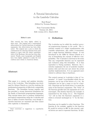
5we want to apply f to a three times we apply thefunction 3 to the arguments f and a yielding:of the function s on z. If we want to add say2 and 3, we just apply the successor function twotimes to 3.3f a (λs.λz.s(s(sz)))f a f (f (f a)).This way of defining numbers provides us with alanguage construct similar to an instruction suchas “FOR i 1 to 3” in other languages. The number zero applied to the arguments f and a yields0f a (λs.λz.z)f a a. That is, applying thefunction f to the argument a zero times leavesthe argument a unchanged.Our first interesting function, after having definedthe natural numbers, is the successor function.This can be defined asS λn.λa.λb.a(nab).The definition looks awkward but it works. Forexample, the successor function applied to ourrepresentation for zero is the expression:S0 (λn.λa.λb.a(nab))0In the body of the first expression, we substitutethe occurrence of n with 0, and then in two steps,0ab reduces to b. This sequence therefore producesthe reduced expressionS0 λa.λb.a(0ab) λa.λb.a(b) 1That is, the result is the representation of thenumber 1 (remember that bound variable namesare “dummies” and can be changed).Successor applied to 1 yields:S1 (λn.λa.λb.a(nab))1 λa.λb.a(1ab) λa.λb.a(ab) 2Notice that the only purpose of applying the number 1 (λs.λz.sz) to the arguments a and b is to“rename” the variables used internally in the definition of our number.2.1AdditionAddition can be obtained immediately by notingthat the body sz of our definition of the number 1,for example, can be interpreted as the applicationLet us try the following in order to compute 2 3:2S3 (λs.λz.s(sz)))S3 S(S3) · · · 5In general m plus n can be computed by the expression mSn.2.2MultiplicationThe multiplication of two numbers x and y can becomputed using the following function:(λx.λy.λa.x(ya))The product of 3 by 3 is then(λx.λy.λa.x(ya))33which reduces to(λa.3(3a))Using the definition of the number 3, we furtherreduce the above expression to(λa.(λs.λb.s(s(sb)))(3a)) (λa.λb.(3a)((3a)((3a)b)))In order to understand why this function reallycomputes the product of 3 by 3, let us look at somediagrams. The first application (3a) is computedon the left of Fig. 4. Notice that the applicationof 3 to a has the effect of producing a new function which applies a three times to the function’sargument.Now, applying the function 3 to the result of (3a)produces three copies of the function obtained inFig. 4 , concatenated as shown on the right inFig. 4 (where the result has been applied to b forclarity). Notice that we have a “tower” of threetimes the same function, each one absorbing thelower one as argument for the application of thefunction a three times, for a total of nine applications.
6(λ sz.s(s(sz)))a(λ ab.(3a)((3a)((3a)b)))aaaathreeapplica onsofsaaaaaaaaaappliedthree mesabaapplied3by3 mestoba(a(a(a(a(a(a(a(ab))))))))At the top of the figure, thenonstandard notation means(λs.λz.s(s(sz)))a.The number 3 applied to argument a produces a new function.At the top, the nonstandard notationmeans (λa.λb.(3a)((3a)((3a)b))).The plumbing of the function 3 applied to 3a, and the result to b.Figure 4: 3 times 33ConditionalsWe introduce the following two functions whichwe call the values “true”T λx.λy.xand “false”The AND function of two arguments can be defined as λx.λy.xyFThis definition works because given that x is true,the truth value of the AND operation depends onthe truth value of y. If x is false (and selects thusthe second argument in xyF) the complete ANDis false, regardless of the value of y.F λx.λy.yThe first function takes two arguments and returns the first one. The second function returnsthe second of two arguments.3.1Logical operationsThe OR function of two arguments can be definedas λx.λy.xTyHere, if x is true, the OR is true. If x is false, itpicks the second argument y and the value of theOR function depends now on the value of y.Negation of one argument can be defined asIt is now possible to define logical operations usingthis representation of the truth values. λx.xFT
7For example, the negation function applied to“true” is T (λx.xFT)Twhich reduces toTFT (λc.λd.c)FT Fthat is, the truth value “false”.Armed with these three logic functions, we can encode any other logic function and reproduce anygiven circuit without feedback (we look at feedback when we deal with recursion).3.23.3The predecessor functionWe can now define the predecessor function combining some of the functions introduced above.When looking for the predecessor of n, the general strategy will be to create a pair (n, n 1) andthen pick the second element of the pair as theresult.A pair (a, b) can be represented in λ-calculus usingthe function(λz.zab)We can extract the first element of the pair fromthe expression applying this function to the continuation λx.λy.x:A conditional test(λz.zab)(λx.λy.x) (λx.λy.x)ab (λy.a)b a,It is very convenient in a programming languageto have a function which is true if a number iszero and false otherwise. The following functionZ fulfills this role:and the second applying the function to continuation λx.λy.y:Z λx.xF FThe following function generates from the pair(n, n 1) (which is the argument p in the function)the pair (n 1, n):To understand how this function works, rememberthat0f a (λs.λz.z)f a athat is, the function f applied zero times to theargument a yields a. On the other hand, F appliedto any argument yields the identity functionFa (λx.λy.y)a λy.y IWe can now test if the function Z works correctly.The function applied to zero yields(λz.zab)(λx.λy.y) (λx.λy.y)ab (λy.y)b b.Φ (λp.λz.z(S(p(λx.λy.x)))(p(λx.λy.x)))The subexpression p(λx.λy.x) extracts the first element from the pair p. A new pair is formed usingthis element, which is incremented for the firstposition of the new pair and just copied for thesecond position of the new pair.The predecessor of a number n is obtained by applying function Φ n times to the pair (λ.z00) andthen selecting the second member of the new pair:Z0 (λx.xF F)0 0F F F TP (λn.(nΦ(λz.z00))(λx.λy.y))because F applied 0 times to yields . The function Z applied to any other number N yieldsZN (λx.xF F)N NF FThe function F is then applied N times to . ButF applied to anything is the identity (as shownbefore), so that the above expression reduces, forany number N greater than zero, toIF FNotice that using this approach the predecessorof zero is zero. This property is useful for thedefinition of other functions.3.4Equality and inequalitiesWith the predecessor function as the buildingblock, we can now define a function which tests
8if a number x is greater than or equal to a number y:G (λx.λy.Z(xPy))times to the recursive call (the argument r) of thefunction applied to the predecessor of n.If the predecessor function applied x times to yyields zero, then it is true that x y.How do we know that r in the expression aboveis the recursive call to R, since functions in λcalculus do not have names? We do not knowand that is precisely why we have to use the recursion operator Y. Assume for example that wewant to add the numbers from 0 to 3. The necessary operations are performed by the call:If x y and y x, then x y. This leads to thefollowing definition of the function E which testsif two numbers are equal:E (λx.λy. (Z(xPy))(Z(yPx)))In a similar manner we can define functions to testwhether x y, x y or x 6 y.4RecursionRecursive functions can be defined in the λcalculus using a function which calls a function yand then regenerates itself. This can be better understood by considering the following function Y:Y (λy.(λx.y(xx))(λx.y(xx)))YR3 R(YR)3 Z30(3S(YR(P3)))Since 3 is not equal to zero, the evaluation is equivalent to3S(YR(P3))that is, the sum of the numbers from 0 to 3 isequal to 3 plus the sum of the numbers from 0to the predecessor of 3 (that is, two). Successiverecursive evaluations of YR will lead to the correctfinal result.Notice that in the function defined above the recursion will be stopped when the argument becomes 0. The final result will beThis function applied to a function R yields:YR (λx.R(xx))(λx.R(xx))3S(2S(1S0))that is, the number 6.which further reduced yieldsR((λx.R(xx))(λx.R(xx))but this means that YR R(YR), that is, thefunction R is evaluated using the recursive call YRas the first argument.An infinite loop, for example, can be programmedas YI, since this reduces to I(YI), then to YI andso ad infinitum.A more useful function is one which adds the firstn natural numbers.We canuse a recursive defiPnPn 1nition, since i 0 i n i 0 i. Let us use thefollowing definition for R:R (λr.λn.Zn0(nS(r(Pn))))This definition tells us that the number n is tested:if it is zero the result of the sum is zero. If n isnot zero, then the successor function is applied n5Projects for the reader1. Define the functions “less than” and “greaterthan” of two numerical arguments.2. Define the positive and negative integers using pairs of natural numbers.3. Define addition and subtraction of integers.4. Define the division of positive integers recursively.5. Define the function n! n · (n 1) · · · 1 recursively.6. Define the rational numbers as pairs of integers.7. Define functions for the addition, subtraction,multiplication and division of rationals.
98. Define a data structure to represent a list ofnumbers.9. Define a function which extracts the first element from a list.10. Define a recursive function which counts thenumber of elements in a list.11. Can you simulate a Turing machine using λcalculus?References[1] P.M. Kogge, The Architecture of SymbolicComputers, McGraw-Hill, New york 1991,chapter 4.[2] G. Michaelson, An Introduction to FunctionalProgramming through λ-calculus, AddisonWesley, Wokingham, 1988.[3] G. Revesz, Lambda-Calculus Combinators andFunctional Programming, Cambridge University Press, Cambridge, 1988, chapters 1-3.
A Tutorial Introduction to the Lambda Calculus Raul Rojas (Edited by Norman Ramsey) Freie Universit at Berlin Version 2.0, 2015 Edit version 2.0-1, March 2018 Editor's note This tutorial has been lightly edited in three ways. The original uses a nonstandard abbreviation for Curried functions of multiple arguments; this abbreviation has been .