Transcription
SAS/OR 13.2 User’s Guide:Mathematical ProgrammingThe QuadraticProgramming Solver
This document is an individual chapter from SAS/OR 13.2 User’s Guide: Mathematical Programming.The correct bibliographic citation for the complete manual is as follows: SAS Institute Inc. 2014. SAS/OR 13.2 User’s Guide:Mathematical Programming. Cary, NC: SAS Institute Inc.Copyright 2014, SAS Institute Inc., Cary, NC, USAAll rights reserved. Produced in the United States of America.For a hard-copy book: No part of this publication may be reproduced, stored in a retrieval system, or transmitted, in any form or byany means, electronic, mechanical, photocopying, or otherwise, without the prior written permission of the publisher, SAS InstituteInc.For a Web download or e-book: Your use of this publication shall be governed by the terms established by the vendor at the timeyou acquire this publication.The scanning, uploading, and distribution of this book via the Internet or any other means without the permission of the publisher isillegal and punishable by law. Please purchase only authorized electronic editions and do not participate in or encourage electronicpiracy of copyrighted materials. Your support of others’ rights is appreciated.U.S. Government License Rights; Restricted Rights: The Software and its documentation is commercial computer softwaredeveloped at private expense and is provided with RESTRICTED RIGHTS to the United States Government. Use, duplication ordisclosure of the Software by the United States Government is subject to the license terms of this Agreement pursuant to, asapplicable, FAR 12.212, DFAR 227.7202-1(a), DFAR 227.7202-3(a) and DFAR 227.7202-4 and, to the extent required under U.S.federal law, the minimum restricted rights as set out in FAR 52.227-19 (DEC 2007). If FAR 52.227-19 is applicable, this provisionserves as notice under clause (c) thereof and no other notice is required to be affixed to the Software or documentation. TheGovernment’s rights in Software and documentation shall be only those set forth in this Agreement.SAS Institute Inc., SAS Campus Drive, Cary, North Carolina 27513.August 2014SAS provides a complete selection of books and electronic products to help customers use SAS software to its fullest potential. Formore information about our offerings, visit support.sas.com/bookstore or call 1-800-727-3228.SAS and all other SAS Institute Inc. product or service names are registered trademarks or trademarks of SAS Institute Inc. in theUSA and other countries. indicates USA registration.Other brand and product names are trademarks of their respective companies.
Gain Greater Insight into YourSAS Software with SAS Books. Discover all that you need on your journey to knowledge and empowerment.support.sas.com/bookstorefor additional books and resources.SAS and all other SAS Institute Inc. product or service names are registered trademarks or trademarks of SAS Institute Inc. in the USA and other countries. indicates USA registration. Other brand and product names aretrademarks of their respective companies. 2013 SAS Institute Inc. All rights reserved. S107969US.0613
Chapter 11The Quadratic Programming SolverContentsOverview: QP Solver . . . . . . . . . . . . . . . . . . . .Getting Started: QP Solver . . . . . . . . . . . . . . . . .Syntax: QP Solver . . . . . . . . . . . . . . . . . . . . .Functional Summary . . . . . . . . . . . . . . . . .QP Solver Options . . . . . . . . . . . . . . . . . .Details: QP Solver . . . . . . . . . . . . . . . . . . . . .Interior Point Algorithm: Overview . . . . . . . . .Parallel Processing . . . . . . . . . . . . . . . . . .Iteration Log . . . . . . . . . . . . . . . . . . . . .Problem Statistics . . . . . . . . . . . . . . . . . .Macro Variable OROPTMODEL . . . . . . . . .Examples: QP Solver . . . . . . . . . . . . . . . . . . . .Example 11.1: Linear Least Squares Problem . . .Example 11.2: Portfolio Optimization . . . . . . .Example 11.3: Portfolio Selection with TransactionsReferences . . . . . . . . . . . . . . . . . . . . . . . . verview: QP SolverThe OPTMODEL procedure provides a framework for specifying and solving quadratic programs.Mathematically, a quadratic programming (QP) problem can be stated as follows:minsubject to12xT Qx C cT xAx f ; D; g bl x uwhereQAxcblu2222222Rn nRm nRnRnRmRnRnis the quadratic (also known as Hessian) matrixis the constraints matrixis the vector of decision variablesis the vector of linear objective function coefficientsis the vector of constraints right-hand sides (RHS)is the vector of lower bounds on the decision variablesis the vector of upper bounds on the decision variables
536 F Chapter 11: The Quadratic Programming SolverThe quadratic matrix Q is assumed to be symmetric; that is,qij D qj i ;8i; j D 1; : : : ; nIndeed, it is easy to show that even if Q 6D QT , then the simple modificationQ D 1 .Q C QT /Q2Q hence symmetry is assumed. When you specify aproduces an equivalent formulation xT Qx xT QxIquadratic matrix, it suffices to list only lower triangular coefficients.In addition to being symmetric, Q is also required to be positive semidefinite for minimization type of models:xT Qx 0;8x 2 RnQ is required to be negative semidefinite for maximization type of models. Convexity can come as a result ofa matrix-matrix multiplicationQ D LLTor as a consequence of physical laws, and so on. See Figure 11.1 for examples of convex, concave, andnonconvex objective functions.Figure 11.1 Examples of Convex, Concave, and Nonconvex Objective FunctionsThe order of constraints is insignificant. Some or all components of l or u (lower and upper bounds,respectively) can be omitted.
Getting Started: QP Solver F 537Getting Started: QP SolverConsider a small illustrative example. Suppose you want to minimize a two-variable quadratic functionf .x1 ; x2 / on the nonnegative quadrant, subject to two constraints:min 2x1 C 3x2subject to x1x2x1 C 2x2x1x2C x12 C 10x22 C 2:5x1 x2 1 100 0 0To use the OPTMODEL procedure, it is not necessary to fit this problem into the general QP formulationmentioned in the section “Overview: QP Solver” on page 535 and to compute the corresponding parameters.However, since these parameters are closely related to the data set that is used by the OPTQP procedureand has a quadratic programming system (QPS) format, you can compute these parameters as follows. Thelinear objective function coefficients, vector of right-hand sides, and lower and upper bounds are identifiedimmediately as 210C1cD; bD; lD; uD31000C1Carefully construct the quadratic matrix Q. Observe that you can use symmetry to separate the main-diagonaland off-diagonal elements:nnX1 T1 X1Xxi qij xjx Qx xi qij xj Dqi i xi2 C222i;j D1i D1i jThe first expressionn1Xqi i xi22i D1sums the main-diagonal elements. Thus, in this case you haveq11 D 2;q22 D 20Notice that the main-diagonal values are doubled in order to accommodate the 1/2 factor. Now the secondtermXxi qij xji jsums the off-diagonal elements in the strict lower triangular part of the matrix. The only off-diagonal(xi xj ; i 6D j ) term in the objective function is 2:5 x1 x2 , so you haveq21 D 2:5Notice that you do not need to specify the upper triangular part of the quadratic matrix.
538 F Chapter 11: The Quadratic Programming SolverFinally, the matrix of constraints is as follows: 11AD12The following OPTMODEL program formulates the preceding problem in a manner that is very close to themathematical specification of the given problem:/* getting started */proc optmodel;var x1 0; /* declare nonnegative variable x1 */var x2 0; /* declare nonnegative variable x2 *//* objective: quadratic function f(x1, x2) */minimize f /* the linear objective function coefficients */2 * x1 3 * x2 /* quadratic x, Qx */x1 * x1 2.5 * x1 * x2 10 * x2 * x2;/* subject to the following constraints */con r1: x1 - x2 1;con r2: x1 2 * x2 100;/* specify iterative interior point algorithm (QP)* in the SOLVE statement */solve with qp;/* print the optimal solution */print x1 x2;save qps qpsdata;quit;The “with qp” clause in the SOLVE statement invokes the QP solver to solve the problem. The output isshown in Figure 11.2.
Getting Started: QP Solver F 539Figure 11.2 Summaries and Optimal SolutionThe OPTMODEL ProcedureProblem SummaryObjective SenseMinimizationObjective FunctionfObjective TypeQuadraticNumber of Variables2Bounded Above0Bounded Below2Bounded Below and Above0Free0Fixed0Number of Constraints2Linear LE ( )1Linear EQ ( )0Linear GE ( )1Linear Range0Constraint Coefficients4Performance InformationExecution ModeSingle-MachineNumber of Threads 4Solution SummarySolverQPAlgorithmInterior PointObjective FunctionfSolution StatusOptimalObjective Value15018Primal Infeasibility 7.034728E-17Dual InfeasibilityBound InfeasibilityDuality ons06Presolve Time0.00Solution Time0.02x1 x234 33In this example, the SAVE QPS statement is used to save the QP problem in the QPS-format data set qpsdata,shown in Figure 11.3. The data set is consistent with the parameters of general quadratic programming
540 F Chapter 11: The Quadratic Programming Solverpreviously computed. Also, the data set can be used as input to the OPTQP procedure.Figure 11.3 QPS-Format Data SetObs FIELD1FIELD2 FIELD3 FIELD4 FIELD5 FIELD61 NAMEqpsdata2 ROWS.3 Nf.4 Lr1.5 Gr2.6 COLUMNS.7x1f2.0 r118x1r21.0.9x2f3.0 r110x2r22.0.11 .5.17x2x220.0.14 QSECTION18 ENDATASyntax: QP SolverThe following statement is available in the OPTMODEL procedure:SOLVE WITH QP / options ;Functional SummaryTable 11.1 summarizes the list of options available for the SOLVE WITH QP statement, classified by function.Table 11.1 Options for the QP SolverDescriptionControl OptionsSpecifies the frequency of printing solution progressSpecifies the maximum number of iterationsSpecifies the time limit for the optimization processSpecifies the type of presolveInterior Point Algorithm OptionsSpecifies the stopping criterion based on duality gapSpecifies the stopping criterion based on dual infeasibilityOptionLOGFREQ MAXITER MAXTIME PRESOLVER STOP DG STOP DI
QP Solver Options F 541Table 11.1 (continued)DescriptionOptionSpecifies the stopping criterion based on primal infea- STOP PI sibilitySpecifies units of CPU time or real timeTIMETYPE QP Solver OptionsThis section describes the options recognized by the QP solver. These options can be specified after a forwardslash (/) in the SOLVE statement, provided that the QP solver is explicitly specified using a WITH clause.The QP solver does not provide an intermediate solution if the solver terminates before reaching optimality.Control OptionsLOGFREQ kPRINTFREQ kspecifies that the printing of the solution progress to the iteration log is to occur after every k iterations.The print frequency, k , is an integer between zero and the largest four-byte signed integer, which is231 1.The value k 0 disables the printing of the progress of the solution. The default value of this option is1.MAXITER kspecifies the maximum number of iterations. The value k can be any integer between one and thelargest four-byte signed integer, which is 231 1. If you do not specify this option, the procedure doesnot stop based on the number of iterations performed.MAXTIME tspecifies an upper limit of t units of time for the optimization process, including problem generationtime and solution time. The value of the TIMETYPE option determines the type of units used. If youdo not specify the MAXTIME option, the solver does not stop based on the amount of time elapsed.The value of t can be any positive number; the default value is the positive number that has the largestabsolute value that can be represented in your operating environment.PRESOLVER number stringPRESOL number stringspecifies one of the following presolve isables presolver.Applies presolver by using default setting.You can specify the PRESOLVER value either by a character-valued option or by an integer. Thedefault option is AUTOMATIC.
542 F Chapter 11: The Quadratic Programming SolverInterior Point Algorithm OptionsSTOP DG ıspecifies the desired relative duality gap, ı 2 [1E–9, 1E–4]. This is the relative difference between theprimal and dual objective function values and is the primary solution quality parameter. The defaultvalue is 1E–6. See the section “Interior Point Algorithm: Overview” on page 543 for details.STOP DI ˇspecifies the maximum allowed relative dual constraints violation, ˇ 2 [1E–9, 1E–4]. The defaultvalue is 1E–6. See the section “Interior Point Algorithm: Overview” on page 543 for details.STOP PI specifies the maximum allowed relative bound and primal constraints violation, 2 [1E–9, 1E–4]. Thedefault value is 1E–6. See the section “Interior Point Algorithm: Overview” on page 543 for details.TIMETYPE number j stringspecifies the units of time used by the MAXTIME option and reported by the PRESOLVE TIME andSOLUTION TIME terms in the OROPTMODEL macro variable. Table 11.3 describes the validvalues of the TIMETYPE option.Table 11.3 Values for TIMETYPE Optionnumber stringDescription01CPUREALSpecifies units of CPU time.Specifies units of real time.The “Optimization Statistics” table, an output of the OPTMODEL procedure if you specify PRINTLEVEL 2 in the PROC OPTMODEL statement, also includes the same time units for Presolver Timeand Solver Time. The other times (such as Problem Generation Time) in the “Optimization Statistics”table are also in the same units.The default value of the TIMETYPE option depends on the value of the NTHREADS option in thePERFORMANCE statement of the OPTMODEL procedure. Table 11.4 describes the detailed logicfor determining the default; the first context in the table that applies determines the default value. Formore information about the NTHREADS option, see the section “PERFORMANCE Statement” onpage 23 in Chapter 4, “Shared Concepts and Topics.”Table 11.4 Default Value for TIMETYPE OptionContextSolver is invoked in an OPTMODEL COFOR loopNTHREADS value is greater than 1NTHREADS 1DefaultREALREALCPU
Details: QP Solver F 543Details: QP SolverInterior Point Algorithm: OverviewThe QP solver implements an infeasible primal-dual predictor-corrector interior point algorithm. To illustratethe algorithm and the concepts of duality and dual infeasibility, consider the following QP formulation (theprimal):min 21 xT Qx C cT xsubject to Ax bx 0The corresponding dual formulation ismaxsubject to1 T2 x QxQxC bT yC AT y C w D cy 0w 0where y 2 Rm refers to the vector of dual variables and w 2 Rn refers to the vector of dual slack variables.The dual makes an important contribution to the certificate of optimality for the primal. The primal anddual constraints combined with complementarity conditions define the first-order optimality conditions, alsoknown as KKT (Karush-Kuhn-Tucker) conditions, which can be stated as follows where e .1; : : : ; 1/T ofappropriate dimension and s 2 Rm is the vector of primal slack variables:Ax sQx C AT y C wWXeSYex; y; w; sDDDD b .primal feasibility/c.dual feasibility/0 .complementarity/0 .complementarity/0N OTE : Slack variables (the s vector) are automatically introduced by the solver when necessary; it is thereforerecommended that you not introduce any slack variables explicitly. This enables the solver to handle slackvariables much more efficiently.
544 F Chapter 11: The Quadratic Programming SolverThe letters X; Y; W; and S denote matrices with corresponding x, y, w, and s on the main diagonal and zeroelsewhere, as in the following example:23x1 0 06 0 x2 0 767X 6 ::: : ::: 74 ::::: 500 xnIf .x ; y ; w ; s / is a solution of the previously defined system of equations that represent the KKTconditions, then x is also an optimal solution to the original QP model.At each iteration the interior point algorithm solves a large, sparse system of linear equations, Y 1SA y„DATQ X 1W x‚where x and y denote the vector of search directions in the primal and dual spaces, respectively, and ‚and „ constitute the vector of the right-hand sides.The preceding system is known as the reduced KKT system. The QP solver uses a preconditioned quasiminimum residual algorithm to solve this system of equations efficiently.An important feature of the interior point algorithm is that it takes full advantage of the sparsity in theconstraint and quadratic matrices, thereby enabling it to efficiently solve large-scale quadratic programs.The interior point algorithm works simultaneously in the primal and dual spaces. It attains optimality whenboth primal and dual feasibility are achieved and when complementarity conditions hold. Therefore, it is ofinterest to observe the following four measures where kvk2 is the Euclidean norm of the vector v: relative primal infeasibility measure : DkAx b sk2kbk2 C 1 relative dual infeasibility measure ˇ:ˇDkQx C c AT ykck2 C 1wk2 relative duality gap ı:ıDjxT Qx C cT xbT yjj 12 xT Qx C cT xj C 1 absolute complementarity :DnXi D1xi wi CmXyi sii D1These measures are displayed in the iteration log.
Parallel Processing F 545Parallel ProcessingThe interior point algorithm can be run in single-machine mode (in single-machine mode, the computation isexecuted by multiple threads on a single computer). You can specify options for parallel processing in thePERFORMANCE statement, which is documented in the section “PERFORMANCE Statement” on page 23in Chapter 4, “Shared Concepts and Topics.”Iteration LogThe following information is displayed in the iteration log:Iterindicates the iteration number.Complementindicates the (absolute) complementarity.Duality Gapindicates the (relative) duality gap.Primal Infeasindicates the (relative) primal infeasibility measure.Bound Infeasindicates the (relative) bound infeasibility measure.Dual Infeasindicates the (relative) dual infeasibility measure.Timeindicates the time elapsed (in seconds).If the sequence of solutions converges to an optimal solution of the problem, you should see all columnsin the iteration log converge to zero or very close to zero. Nonconvergence can be the result of insufficientiterations being performed to reach optimality. In this case, you might need to increase the value that youspecify in the MAXITER or MAXTIME option. If the complementarity or the duality gap does notconverge, the problem might be infeasible or unbounded. If the infeasibility columns do not converge, theproblem might be infeasible.Problem StatisticsOptimizers can encounter difficulty when solving poorly formulated models. Information about datamagnitude provides a simple gauge to determine how well a model is formulated. For example, a modelwhose constraint matrix contains one very large entry (on the order of 109 ) can cause difficulty when theremaining entries are single-digit numbers. The PRINTLEVEL 2 option in the OPTMODEL procedurecauses the ODS table ProblemStatistics to be generated when the QP solver is called. This table providesbasic data magnitude information that enables you to improve the formulation of your models.The example output in Figure 11.4 demonstrates the contents of the ODS table ProblemStatistics.
546 F Chapter 11: The Quadratic Programming SolverFigure 11.4 ODS Table ProblemStatisticsThe OPTMODEL ProcedureProblem StatisticsNumber of Constraint Matrix Nonzeros4Maximum Constraint Matrix Coefficient2Minimum Constraint Matrix Coefficient1Average Constraint Matrix Coefficient1.25Number of Linear Objective Nonzeros2Maximum Linear Objective Coefficient3Minimum Linear Objective Coefficient2Average Linear Objective Coefficient2.5Number of Lower Triangular Hessian Nonzeros1Number of Diagonal Hessian Nonzeros2Maximum Hessian CoefficientMinimum Hessian CoefficientAverage Hessian CoefficientNumber of RHS NonzerosMaximum RHSMinimum RHSAverage RHS2026.752100150.5Maximum Number of Nonzeros per Column2Minimum Number of Nonzeros per Column2Average Number of Nonzeros per Column2Maximum Number of Nonzeros per Row2Minimum Number of Nonzeros per Row2Average Number of Nonzeros per Row2Macro Variable OROPTMODELThe OPTMODEL procedure always creates and initializes a SAS macro called OROPTMODEL . Thisvariable contains a character string. After each PROC OROPTMODEL run, you can examine this macro byspecifying %put & OROPTMODEL ; and check the execution of the most recently invoked solver from thevalue of the macro variable. The various terms of the variable after the QP solver is called are interpreted asfollows.STATUSindicates the solver status at termination. It can take one of the following values:OKThe solver terminated normally.SYNTAX ERRORIncorrect syntax was used.DATA ERRORThe input data were inconsistent.
Macro Variable OROPTMODEL F 547OUT OF MEMORYInsufficient memory was allocated to the procedure.IO ERRORA problem occurred in reading or writing data.SEMANTIC ERRORAn evaluation error, such as an invalid operand type, occurred.ERRORThe status cannot be classified into any of the preceding categories.ALGORITHMindicates the algorithm that produced the solution data in the macro variable. This term only appearswhen STATUS OK. It can take the following value:IPThe interior point algorithm produced the solution data.SOLUTION STATUSindicates the solution status at termination. It can take one of the following values:OPTIMALThe solution is optimal.CONDITIONAL OPTIMALThe solution is optimal, but some infeasibilities (primal,dual or bound) exceed tolerances due to scaling or preprocessing.INFEASIBLEThe problem is infeasible.UNBOUNDEDThe problem is unbounded.INFEASIBLE OR UNBOUNDEDThe problem is infeasible or unbounded.BAD PROBLEM TYPEThe problem type is unsupported by the solver.ITERATION LIMIT REACHEDThe maximum allowable number of iterations wasreached.TIME LIMIT REACHEDThe solver reached its execution time limit.FUNCTION CALL LIMIT REACHEDThe solver reached its limit on function evaluations.INTERRUPTEDThe solver was interrupted externally.FAILEDThe solver failed to converge, possibly due to numericalissues.OBJECTIVEindicates the objective value obtained by the solver at termination.PRIMAL INFEASIBILITYindicates the (relative) infeasibility of the primal constraints at the solution. See the section “InteriorPoint Algorithm: Overview” on page 543 for details.DUAL INFEASIBILITYindicates the (relative) infeasibility of the dual constraints at the solution. See the section “InteriorPoint Algorithm: Overview” on page 543 for details.
548 F Chapter 11: The Quadratic Programming SolverBOUND INFEASIBILITYindicates the (relative) violation by the solution of the lower or upper bounds (or both). See the section“Interior Point Algorithm: Overview” on page 543 for details.DUALITY GAPindicates the (relative) duality gap. See the section “Interior Point Algorithm: Overview” on page 543for details.COMPLEMENTARITYindicates the (absolute) complementarity at the solution. See the section “Interior Point Algorithm:Overview” on page 543 for details.ITERATIONSindicates the number of iterations required to solve the problem.PRESOLVE TIMEindicates the time taken for preprocessing (in seconds).SOLUTION TIMEindicates the time (in seconds) taken to solve the problem, including preprocessing time.N OTE : The time that is reported in PRESOLVE TIME and SOLUTION TIME is either CPU time or realtime. The type is determined by the TIMETYPE option.Examples: QP SolverThis section presents examples that illustrate the use of the OPTMODEL procedure to solve quadraticprogramming problems. Example 11.1 illustrates how to model a linear least squares problem and solve itby using PROC OPTMODEL. Example 11.2 and Example 11.3 show in detail how to model the portfoliooptimization and selection problems.Example 11.1: Linear Least Squares ProblemThe linear least squares problem arises in the context of determining a solution to an overdetermined setof linear equations. In practice, these equations could arise in data fitting and estimation problems. Anoverdetermined system of linear equations can be defined asAx D bwhere A 2 Rm n , x 2 Rn , b 2 Rm , and m n. Since this system usually does not have a solution, youneed to be satisfied with some sort of approximate solution. The most widely used approximation is the leastsquares solution, which minimizes kAx bk22 .This problem is called a least squares problem for the following reason. Let A, x, and b be defined aspreviously. Let ki .x/ be the kth component of the vector Ax b:ki .x/ D ai1 x1 C ai 2 x2 C C ai n xnbi ; i D 1; 2; : : : ; m
Example 11.1: Linear Least Squares Problem F 549By definition of the Euclidean norm, the objective function can be expressed as follows:kAxbk22DmXki .x/2i D1Therefore, the function you minimize is the sum of squares of m terms ki .x/; hence the term least squares.The following example is an illustration of the linear least squares problem; that is, each of the terms ki is alinear function of x .Consider the following least squares problem defined by232 34 014541 1 ; bD 0 5AD3 21This translates to the following set of linear equations:4x1 D 1;x1 C x2 D 0;3x1 C 2x2 D 1The corresponding least squares problem is:minimize .4x11/2 C . x1 C x2 /2 C .3x1 C 2x21/2The preceding objective function can be expanded to:minimize 26x12 C 5x22 C 10x1 x214x14x2 C 2In addition, you impose the following constraint so that the equation 3x1 C 2x2 D 1 is satisfied within atolerance of 0.1:0:9 3x1 C 2x2 1:1You can use the following SAS statements to solve the least squares problem:/* example 1: linear least-squares problem */proc optmodel;var x1; /* declare free (no explicit bounds) variable x1 */var x2; /* declare free (no explicit bounds) variable x2 *//* declare slack variable for ranged constraint */var w 0 0.2;/* objective function: minimize is the sum of squares */minimize f 26 * x1 * x1 5 * x2 * x2 10 * x1 * x2- 14 * x1 - 4 * x2 2;/* subject to the following constraint */con L: 3 * x1 2 * x2 - w 0.9;solve with qp;/* print the optimal solution */print x1 x2;quit;The output is shown in Output 11.1.1.
550 F Chapter 11: The Quadratic Programming SolverOutput 11.1.1 Summaries and Optimal SolutionThe OPTMODEL ProcedureProblem SummaryObjective SenseMinimizationObjective FunctionfObjective TypeQuadraticNumber of Variables3Bounded Above0Bounded Below0Bounded Below and Above1Free2Fixed0Number of Constraints1Linear LE ( )0Linear EQ ( )1Linear GE ( )0Linear Range0Constraint Coefficients3Performance InformationExecution ModeSingle-MachineNumber of Threads 4Solution SummarySolverQPAlgorithmInterior PointObjective FunctionfSolution StatusOptimalObjective Value0.0095238095Primal Infeasibility 1.926295E-12Dual Infeasibility1.3056209E-9Bound Infeasibility0Duality ns3Presolve Time0.00Solution Time0.02x1x20.2381 0.1619
Example 11.2: Portfolio Optimization F 551Example 11.2: Portfolio OptimizationConsider a portfolio optimization example. The two competing goals of investment are (1) long-term growthof capital and (2) low risk. A good portfolio grows steadily without wild fluctuations in value. The Markowitzmodel is an optimization model for balancing the return and risk of a portfolio. The decision variables arethe amounts invested in each asset. The objective is to minimize the variance of the portfolio’s total return,subject to the constraints that (1) the expected growth of the portfolio reaches at least some target level and(2) you do not invest more capital than you have.Let x1 ; : : : ; xn be the amount invested in each asset, B be the amount of capital you have, R be the randomvector of asset returns over some period, and r be the expected value of R. Let G be the minimum growthnPyou hope to obtain, and C be the covariance matrix of R. The objective function is Varxi Ri , whichi D1can be equivalently denoted as xT Cx.Assume, for example, n 4. Let B 10,000, G 1,000, r D Œ0:05; 0:2; 0:15; 0:30 , and230:080:050:050:056 0:05 0:160:020:02 77C D 64 0:050:02 0:350:06 50:050:02 0:060:35The QP formulation can be written as:min 0:08x12 0:1x1 x2 0:1x1 x3 0:1x1 x4 C 0:16x220:04x2 x3 0:04x2 x4 C 0:35x32 C 0:12x3 x4 C 0:35x42subject to.budget/.growth/ 0:05x1x1 C x2 C x3 C x4 100000:2x2 C 0:15x3 C 0:30x4 1000x1 ; x2 ; x3 ; x4 0Use the following SAS statements to solve the problem:/* example 2: portfolio optimization */proc optmodel;/* let x1, x2, x3, x4 be the amount invested in each asset */var x{1.4} 0;num coeff{1.4, 1.4} [0.08 -.05-.05 0.16-.05 -.02-.05 -.02num r{1.4} [0.05 -.20 0.15 0.30];-.05-.020.350.06-.05-.020.060.35];/* minimize the variance of the portfolio's total return */minimize f sum{i in 1.4, j in 1.4}coeff[i,j]*x[i]*x[j];/* subject to the following constraints */con BUDGET: sum{i in 1.4}x[i] 10000;con GROWTH: sum{i in 1.4}r[i]*x[i] 1000;
552 F Chapter 11: The Quadratic Programming Solversolve with qp;/* print the optimal solution */print x;The summaries and the optimal solution are shown in Output 11.2.1.Output 11.2.1 Portfolio OptimizationThe OPTMODEL ProcedureProblem SummaryObjective SenseMinimizationObjective FunctionfObjective TypeQuadraticNumber of Variables4Bounded Above0Bounded Below4Bounded Below and Above0Free0Fixed0Number of Constraints2Linear LE ( )1Linear EQ ( )0Linear GE ( )1Linear Range0Constraint Coefficients8Performance InformationExecution ModeSingle-MachineNumber of Threads 4Solution SummarySolverAlgorithmObjective FunctionQPInterio
QP Solver Options This section describes the options recognized by the QP solver. These options can be specified after a forward slash (/) in the SOLVE statement, provided that the QP solver is explicitly specified using a WITH clause. The QP solver does not provide an intermediate solution if the solver terminates before reaching optimality.