Transcription
An Adaptive Learning Approach for Noisy Data StreamsFang ChuYizhou WangCarlo ZanioloTechnical Report, TR040029Computer Science Department, UCLA{fchu,wangyz,zaniolo}@cs.ucla.eduAbstractTwo critical challenges typically associated with miningdata streams are concept drift and data contamination. Toaddress these challenges, we seek learning techniques andmodels that are robust to noise and can adapt to changesin timely fashion. In this paper, we approach the streammining problem using a statistical estimation framework,and propose a fast and robust discriminative model forlearning on noisy data streams. We build an ensemble ofclassifiers to achieve timely adaptation by weighting classifiers in a way that maximizes the likelihood of the data. Wefurther employ robust statistical techniques to alleviate theproblem of noise sensitivity. Experimental results on bothsynthetic and real-life data sets demonstrate the effectiveness of this new model learning approach.1. IntroductionThere is much current research interest in continuousmining of data: i.e., data that arrives continuously in highvolume and speed. Applications involving stream dataabound and include network traffic monitoring, credit cardfraud detection and stock market trend analysis. Practicalsituations pose three fundamental issues to be addressed byany continuous mining attempt. Adaptation Issue.In traditional learning tasks, data is stationary andthe underlying concept that maps the attributes toclass labels is unchanging. With data streams, however, the concept is not static but drifts with time dueto changes in the environment. For example, customer purchase preferences alter with seasons, fashion, and the emerging of competing products and services. These changes cause the model learned from olddata obsolete and inconsistent with the new data, andupdating the model becomes necessary. This is commonly known as the concept drift problem [20]. It isconsidered to be one of the core issues of data streammining [8]. Robustness Issue.Data contamination is a serious problem since noisecan severely impair the quality and speed of learning. This problem is encountered in many applicationswhere the source data can be unreliable, and also errorscan be injected during data transmission. This problemis even more challenging for data streams, where it isdifficult to distinguish noise from data caused by concept drift. If an algorithm is too eager to adapt to concept changes, it may overfit noise by mistakenly interpreting it as data from a new concept. If the algorithmis too conservative and slow to adapt, it may overlookimportant changes (and, for instance, miss out on theopportunities created by a timely identification of newtrends in the marketplace). Performance Issue.Constrained by the requirement of on-line responsesand by limited computation and memory resources,continuous data stream mining should conform to thefollowing criteria: (1) learning should be done veryfast, preferably in one pass of the data; and (2) algorithms should make light demands on memory resources, for the storage of either the intermediate results or the final decision models. These “fast andlight” requirements exclude computationally expensive algorithms, such as support vector machines, orvery large models, such as decision trees with thousands of nodes.1.1. Related WorkThe concept drift problem has been addressed in bothmachine learning and data mining communities. The firstsystems capable of handling concept drift were STAGGER[15], ib3 [2] and the FLORA family [20]. These algorithmsprovided valuable insights. But, as they were developed and
tested only on small datasets, they may not be suitable fordata streams which is on a significantly larger scale thanpreviously studied.Several scalable learning algorithms designed for datastreams were proposed recently. They either maintain asingle model incrementally, or an ensemble of base learners. The first category includes Hoeffding tree [10], whichgrows a decision tree node by splitting an attribute onlywhen that attribute is statistically predictive. Hoeffding-treelike algorithms need a large training set in order to reacha fair performance, which makes them unsuitable to situations featuring frequent changes. Domeniconi and Gunopulos [7] designed an incremental support vector machinealgorithm for continuous learning.The second category of scalable learning algorithms areensemble-based approaches. Kolter and Maloof [11] proposed to track concept drift by an ensemble of experts. Thepoor experts are weighted down or discarded, and the goodexperts are updated using recent examples incrementally.Their method is limited to situations where the values ofeach attribute follow a Gaussian distribution. This assumption is necessary to get an efficient incremental algorithm,but not practical in many situations.Other ensemble-based approaches simply partition thedata stream into sequential blocks of fixed size and learn anensemble from these blocks. Base models are constructedonce at a time and never updated incrementally, so that anyoff-the-shelf learning algorithm can be used. These ensembles adopt different voting schemes to reach a final decision. Street et al. [17] let their ensemble vote uniformly,while Wang et al. [18] prefer a weighted voting, assigningclassifier weights proportional to their accuracy on the latestdata block. These two approaches, [17] and [18], are mostclosely related to what we will present in this paper, as ourmethod also builds an ensemble from sequential blocks. Forease of later reference in comparative study, we name themas Bagging and Weighted Bagging, respectively. (The name“bagging” derives from their analogy to traditional baggingensembles [4].)What is missing from the above mentioned work is amechanism for noise identification, or often indistinguishably called outlier detection (as what we will use thereafter). Although there have been a number of off-line algorithms [1, 14, 5, 12, 6] for outlier detection, they are unsuitable for stream data as they assume a single unchanging data model, hence unable to distinguish noise from datacaused by concept drift. In addition, outlier detection withstream data faces general problems such as the choice of adistance metric. Most of the traditional approaches use Euclidean distance, which is unable to treat categorical values.1.2. Our MethodTo address the three above mentioned issues, we propose a novel discriminative model for adaptive learning onnoisy data streams, with modest resource consumption. Fora learnable concept, the class of a sample conditionally follows a Bernoulli distribution. Our method assigns classifierweights in a way that maximizes the training data likelihood with the learned distribution. This weighting schemehas theoretical guarantee for adaptability. In addition, aswe have verified experimentally, our weighting scheme canalso boost a collection of weak classifiers into a strong ensemble. Examples of weak classifiers include decision treeswith very few nodes. It is desirable to use weak classifiersbecause it learns faster and consumes less resources.Our outlier detection differs from previous approaches inthat it is tightly integrated into the adaptive model learning.The motivation is that outliers are directly defined by thecurrent concept, so the outlier identifying strategy needs tobe modified whenever the concept drifts away. In our integrated learning, outliers are defined as samples with a smalllikelihood given the current model, and then the model is refined on the training data with outliers removed. The overalllearning is an iterative process in which the model learningand outlier detection mutually reinforce each other.Another advantage of our outlier detection technique isthe general distance metric for identifying outliers. We define a distance metric based on predictions of the currentensemble, instead of a function in the data space. It canhandle both numerical and categorical values.In section 2 and section 3 we describe the discriminative model with regard to adaptation and robustness, respectively. Section 4 gives the model formulation and computation. Experimental results are shown in section 5.2. Adaptation to Concept DriftEnsemble weighting is the key to fast adaptation. Herewe show that this problem can be formulated as a statisticaloptimization problem solvable by logistic regression.We first look at how an ensemble is constructed andmaintained. The data stream is simply partitioned into smallblocks of fixed size, then classifiers are learned from blocks.The most recent K classifiers comprise the ensemble, andold classifiers retire sequentially by age. Besides a setof training examples for classifier learning, another set oftraining examples are also needed for classifier weighting.If training data is sufficient, we can reserve part of it forweight training; otherwise, randomly sampled training examples can serve the purpose. We only need to make thetwo data sets as synchronized as possible. When sufficienttraining data is collected for classifier learning and ensemble weighting, the following steps are conducted: (1) learn a
new classifier from the training block; (2) replace the oldestclassifier in the ensemble with this newly learned; and then(3) weight the ensemble.The rest of this section gives a formal description of ensemble weighting. A two-class classification setting is considered for simplicity, but the treatment can be extended tomulti-class tasks.The training data for ensemble weighting is representedas(X , Y) {(xi , yi ); i 1, · · · , N }xi is a vector valued sample attribute and yi {0, 1} thesample class label. We assume an ensemble of classifiers,denoted in a vector form asf (f1 (x), · · · , fK (x))Twhere each fk (x) is a classifier function producing a valuefor the belief on a class. The individual classifiers in theensemble may be weak or out-of-date. It is the goal of ourdiscriminative model M to make the ensemble strong byweighted voting. Classifier weights are model parameters,denoted asw (w1 , · · · , wK )Twhere wk is the weight associated with classifier fk . Themodel M also specifies for decision making a weighted voting scheme, that is,wT · fBecause the ensemble prediction wT · f is a continuousvalue, yet the class label yi to be decided is discrete, a standard approach is to assume that yi conditionally follows aBernoulli distribution parameterized by a latent score ηi :yi xi ; f , w Ber(q(ηi ))ηi w T · f(1)Regression is adaptive because it always tries to fit thedata from the current concept. But, it can potentially overfitoutliers. We integrate the following outlier detection technique into the model learning.We define outliers as samples with a small likelihood under a given data model. The goal of learning is to computea model that best fits the bulk of the data, that is, the inliers.Whether a sample is an outlier is hidden information in thisproblem. This suggest us to solve the problem under theEM framework, using a robust statistical formulation.Previously we have described a training data set as{(xi , yi ), i 1, · · · , N }, or (X , Y). This is an incompletedata set, as the outlier information is missing. A completedata set is a triplet(X , Y, Z)whereZ {z1 , · · · , zN }is a hidden variable that distinguishes the outliers from theinliers. zi 1 if (xi , yi ) is an outlier, zi 0 otherwise.This Z is not observable and needs to be inferred. After thevalues of Z are inferred, (X , Y) can be partitioned into aclean sample set(X0 , Y0 ) {(xi , yi , zi ), xi X , yi Y, zi 0}(Xφ , Yφ ) {(xi , yi , zi ), xi X , yi Y, zi 1}eηi1 eηiEq.1 states that yi follows a Bernoulli distribution withparameter q, thus the posterior probability isp(yi xi ; f , w) q yi (1 q)1 yi3. Robustness to Outliersand an outlier setwhere q(ηi ) is the logit transformation of ηi :q(ηi ) , logit(ηi ) our work, we formulate the classifier weighting problem asan optimization problem and solve it using logistic regression. In section 5 we show that such a formulation and solution provide much better adaptability than previous work.(Refer to Fig.1-2, section 5 for a quick reference.)(2)The above description leads to optimizing classifierweights using logistic regression. Given a data set (X , Y)and an ensemble f , the logistic regression technique optimizes the classifier weights by maximizing the likelihoodof the data. The optimization problem has a closed-formsolution which can be quickly solved. We postpone the detailed model computation till section 4.Logistic regression is a well-established regressionmethod, widely used in traditional areas when the regressors are continuous and the responses are discrete [9]. InIt is the samples in (X0 , Y0 ) that all come from one underlying distribution, and are used to fit the model parameters.To infer the outlier indicator Z, we introduce a newmodel parameter λ. It is a threshold value of sample likelihood. A sample is marked as an outlier if its likelihoodfalls below λ. This λ, together with f (classifier functions)and w (classifier weights) discussed earlier, constitutes thecomplete set of parameters of our discriminative model M,denoted as M(x; f , w, λ).4. Model LearningIn this section, we give the model formulation followedby model computation. The symbols used are summarizedin table 1.
(xi , yi )(X , Y)Z(X , Y, Z)(X0 , Y0 )(Xφ , Yφ )Mfwλa sample, with xi the sample attribute, yi thesample class label,an incomplete data set without outlier information,a hidden variable,a complete data set with outlier information,a clean data set,an outlier set,the discriminative model,a vector of classifier function, a model parameter,a vector of classifier weights, a model parameter,a threshold of likelihood, a model parameter.Table 1. Summary of symbols usedAfter expanding the log-likelihood term, we have:log p((X0 , Y0 ) f , w)X log p((xi , yi ) f , w)xi X0 Xxi X0 1. To infer about the hidden variable Z that distinguishesinliers (X0 , Y0 ) from outliers (Xφ , Yφ ).2. To compute the optimal fit for model parameters w andλ in the discriminative model M (x; f , w, λ).Each inlier sample (xi , yi ) (X0 , Y0 ) is assumed to bedrawn from an independent identical distribution belongingto a probability family characterized by parameters w, denoted by a density function p((x, y); f , w). The problemis to find the values of w that maximizes the likelihood of(X0 , Y0 ) in the probability family. As customary, we uselog-likelihood to simplify the computation:log p((X0 , Y0 ) f , w)A parametric model for outlier distribution is not available because outliers are highly irregular. We use insteada non-parametric statistics based on the number of outliers(k(Xφ , Yφ )k). Then, the problem becomes an optimizationproblem. The score function to be maximized involves twoparts: (i) the log-likelihood term for the inliers (X0 , Y0 ),and (ii) a penalty term for the outliers (Xφ , Yφ ). That is:¡(w, λ) arg max log p((X0 , Y0 ) f , w)(w,λ) ζ((Xφ , Yφ ); w, λ)(3)where the penalty term, which penalizes having too manyoutliers, is defined as(4)w and λ affect ζ implicitly. The value of e empiricallydepends on the size of the training data. In our experimentswe set e (0.2, 0.3).log p(xi )xi X0(w,λ)Our model has a four-tuple representationM(x; f , w, λ). Given a training data set (X , Y), anensemble of classifiers f (f1 (x), · · · , fK (x))T , we wantto achieve two objectives.XPAbsorbp(xi ) into the penalty termxi X0 logζ((Xφ , Yφ ); w, λ), and replace the likelihood in Eq.3 withthe logistic form (Eq.2), then the optimization goal becomesfinding the best fit (w, λ) .³ X ¡ yi q (1 yi )(1 q)(w, λ) arg max4.1. Model Formulationζ((Xφ , Yφ ); w, λ) e · k(Xφ , Yφ )klog p(yi xi ; f , w) xi X0 ζ((Xφ , Yφ ); w, λ)(5)The score function to be maximized is not differentiablebecause of the non-parametric penalty term. We have to resort to a more elaborate technique based on the ExpectationMaximization (EM) [3] algorithm to solve the problem.4.2. Inference and ComputationThe main goal of model computation is to infer themissing variables and compute the optimal model parameters, under the EM framework. The EM in general is amethod for maximizing data likelihood in problems wheredata is incomplete. The algorithm iteratively performs anExpectation-Step (E-Step) followed by an MaximizationStep (M-Step) until convergence. In our case,1. E-Step: to impute / infer the outlier indicator Z basedon the current model parameters (w, λ).2. M-Step: to compute new values for (w, λ) that maximize the score function in Eq. 3 with current Z.Next we will discuss how to impute outliers in E-Step,and how to solve the maximization problem in M-Step.The M-Step is actually a Maximum Likelihood Estimation(MLE) problems.E-Step: Impute OutliersWith the current model parameters w (classifierweights), the model for clean data is established as inEq.1, that is, the class label (yi ) of a sample xi followsa Bernoulli distribution parameterized with the ensembleprediction for this sample (wT · f (xi )). Thus, yi ’s loglikelihood p(yi xi ; f , w) can be computed by Eq.2.Note that the line between outliers and inliers is drawnby λ, which is computed in the previous M-Step. So, theformulation of imputing outliers is straightforward:¡ zi sign log p(yi xi ; f , w) λ(6)
½wheresign(x) 1 if x 00 otherwiseM-Step: MLEThe score function (in Eq.5) to be maximized is not differentiable because of the penalty term. We consider a simple approach for an approximate solution. In this approach,the computation of λ and w is separated.1. λ is computed using standard K-means clustering algorithm on log-likelihood p(yi xi ; f , w). In our experiments we choose K 3. The cluster boundaries arecandidates of likelihood threshold λ separating outliers from inliers.2. By fixing each of the candidate λ , w can be computed using the standard MLE procedure. Running aMLE procedure for each candidate λ , and the maximum likelihood will identify the best fit of (w, λ) .The standard MLE procedure for computing w is described as follows. Taking the derivative of the inlier likelihood with respect to w and set it to zero, we have X ¡eηi1 yi (1 yi ) 0ηi w1 e1 eηiyi Y0To solve this equation, we use the Newton-Raphson procedure, which requires the first and second derivatives. Forclarity of notation, we use h(w) to denote the first derivative of inlier likelihood function with regard to w. Startingfrom wt , a single Newton-Raphson update iswt 1 wt ³ 2 h(w ) 1 h(w )tt w wT wHere we haveX h(w) (yi q)f (xi ) wyi Y0and,X 2 h(w) q(1 q)f (xi )f T (xi )T w wyi Y0The initial values of w is important for computation convergence. Since there is no prior knowledge, we can initially set w to be uniform.5. Experiments and DiscussionsWe use both synthetic data and a real-life application toevaluate our discriminative model’s adaptability to conceptshifts and robustness to noise. Our model is compared withthe two previously mentioned approaches: Bagging [17]and Weighted Bagging [18]. We show that although the empirical weighting in Weighted Bagging performs better thanunweighted voting, the robust regression weighting methodis more superior, in terms of both adaptability and robustness.C4.5 decision trees are used in our experiments, but inprinciple our method can be used with any base learningalgorithm.5.1. Data SetsSynthetic DataIn the synthetic data set for controlled study, a sample(x, y) has three independent features x x1 , x2 , x3 ,xi [0, 1], i 0, 1, 2. Geometrically, samples are pointsin a 3-dimension unit cube. The real class boundary is asphere defined asB(x) 2X(xi ci )2 r2 0i 0where c c1 , c2 , c3 is the center of the sphere, r theradius. y 1 if B(x) 0, y 0 otherwise. This learningtask is not easy due to the continuous feature space and thenon-linear class boundary.To simulate a data stream with concept drift, we movethe center c of the sphere that defines the class boundarybetween adjacent blocks. The movement is along each dimension with a step of δ. The value of δ controls thelevel of shifts from small, moderate to large, and the signof δ is randomly assigned independently along each dimension. For example, if a block has c (0.40, 0.60, 0.50),δ 0.05, the sign along each direction is ( 1, 1, 1),then the next block would have c (0.45, 0.55, 0.45). Thevalues of δ ought to be in a reasonable range, to keep theportion of samples that change class labels reasonable. Inour setting, we consider a concept shift small if δ is around0.02, and relatively large if δ around 0.1.To study the model robustness, we insert noise into thetraining data sets by randomly flipping the class labels witha probability of p, p 10%, 15%, 20%. Clean testing datasets are used in all the experiments for accuracy evaluation.Credit Card DataThe real-life application is to build a weighted ensemble for detection of fraudulent transactions in credit cardtransactions, data contributed by a major credit card company. A transaction has 20 features, including the transaction amount, the time of the transaction, and so on. Detaileddata description is given in [16, 18]. Same as in [18], concept drift in our work is simulated by sorting transactionsby the transaction amount.
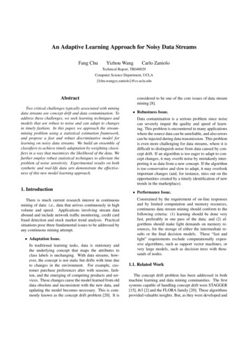
10.950.9Accuracy0.850.80.750.70.65Robust Logistic RegressionWeighted BaggingBagging0.6020406080Data Blocks100120140160Figure 3. Robustness comparison of the three ensemblemethods for different noise levels.Figure 1. Adaptability comparison of the ensemble methods on data with three abrupt shifts.10.950.9Accuracy0.850.80.750.70.65Robust Logistic RegressionWeighted BaggingBagging0.6020406080Data Blocks100120140160Figure 2. Adaptability comparison of the ensemble meth-Figure 4. In the outliers detected, the normalized ratio of(1) true noisy samples (the upper bar), vs. (2) samples froman emerging concept (the lower bar). The bars correspondto blocks 0-59 in the experiments shown in Fig.2ods on data with three abrupt shifts mixed with small shifts.5.2. Evaluation of AdaptationIn this subsection we compare our robust regression ensemble method with Bagging and Weighted Bagging. Concept drift is simulated by moving the class boundary center between adjacent data blocks. The moving distance δalong each dimension controls the magnitude of conceptdrift. We have two sets of experiments with different δvalues, both have abrupt large changes occurring at block40, 80 and 120. In one experiment, data remains stationary between these changing points. In the other experiment, small shifts are mixed between abrupt ones, withδ (0.005, 0.03). The percentage of positive samples fluc-tuates between (41%, 55%). Noise level is 10%.As shown in Fig.1 and Fig.2, the robust regression modelalways gives the best performance. The unweighted bagging ensembles has the worst predictive accuracy. Bothbagging methods are seriously impaired at the conceptchanging points, but the robust regression is able to catchup with the new concept quickly.5.3. Robustness in the Presence of OutliersNoise is the major source of outliers. Fig. 3 shows theensemble performance for the different noise levels: 0%,5%, 10%, 15% and 20%. The accuracy is averaged over 100runs spanning 160 blocks, with small gradual shifts between
10.950.950.90.85AccuracyAverage Accuracy0.90.850.80.750.80.70.750.65Robust Logistic RegressionWeighted BaggingBaggingRobust Logistic RegressionWeighted BaggingBagging0.60.781632fullsize# terminal nodes of base decision trees in ensembles020406080Figure 5. Performance comparison of the ensemble meth-Figure 6. Performance comparison of the ensembles onods with classifiers of different size. Robust regression withsmaller classifiers is compatible to the others with largerclassifiers.credit card data. Base decision trees have no more than 16terminal nodes. Concept shifts are simulated by sorting thetransactions by the transaction amount.blocks. We can make two major observations here:1. The robust regression ensembles are the most accuratefor all the noise levels, as clearly shown in Fig. 3.2. Robust regression also gives the least performancedrops when noise increases. This conclusion is confirmed using paired t-test at 0.05 level. In each casewhen noise level increases by 10%, 15% or 20%, thedecrease in accuracy produced by robust regression isthe smallest, and the differences are statistically significant.To better understand why the robust regression methodis less impacted by outliers, we show the outliers it detectsin Fig.4. Outliers consist mostly noisy samples and samplesfrom a newly emerged concept. In the experiments shownin Fig.2, we record the outliers in blocks 0-59 and calculate the normalized ratio of the two parts. As it shows, truenoise dominates the identified outliers. At block 40 whereconcept drift is large, a bit more samples reflecting the newconcept are mistakenly reported as outliers, but still moretrue noisy samples are identified at the same time.5.4. Discussions on Performance IssueConstrained by the requirement of on-line responses andby limited computation and memory resources, stream datamining methods should learn fast, and produce simple classifiers. For ensemble learning, simple classifiers help toachieve these goals. Here we show that simple decisiontrees can be used in the logistic regression model for better performance.100Data BlocksThe simple classifiers we use are decision trees with 8,16, 32 terminal nodes. Full grown trees are also included forcomparison and denoted as “fullsize” where referred. Fig.5compares the accuracies (averaged over 160 blocks) of theensembles. First to note is that the robust regression methodis always the best despite of the tree size. More importantly,it boosts a collection of simple classifiers, which are weakin classification capability individually, into a strong ensemble. Actually the robust regression ensemble of smallerclassifiers is compatible or even better than the two bagging ensembles of larger classifiers. We observed the abovementioned superior performance of the robust regressionmethod under different levels of noise.For the computation time study, we verify that robustregression is compatible to weighted bagging in terms ofspeed. In a set of experiments where the three methodsrun for about 40 blocks, the learning together with evaluation time totals a 138 seconds for unweighted bagging. Itis 163 seconds for weighted bagging, and 199 seconds forthe robust regression. The running time is obtained whenfull grown decision trees are used. If small decision treesare used instead, logistic regression learning can further besped up yet still perform better than the other two methodswith full grown trees.5.5. Experiments on Real Life DataThe real-life application is to build a classification modelfor detection of fraudulent transactions in credit card transactions. A transaction has 20 features including the transaction amount, the time of the transaction, etc.We study the ensemble performance using differentblock size (1k, 2k, 3k and 4k), and different base mod-
els (decision trees with terminal nodes no more than 8, 16,32 and full-size trees). We show one experiment in Fig.6,where the block size is 1k, and the base models have at most16 terminal nodes. Results of other experiments are similar.The curve shows fewer and smaller drops in accuracy for therobust regression than for the other methods. These dropsoccur when the transaction amount jumps. Overall, the robust regression ensemble method performs better than theother two ensemble methods.6. Summary and Future WorkIn this paper, we propose an adaptive and robust modellearning method that is highly adaptive to concept changesand is robust to noise. The model produces a weighted ensemble. The weights of classifiers are computed by logisticregression technique, which ensures good adaptability. Furthermore, this logistic regression-based weighting schemeis capable to boost a collection of weak classifiers, thusachieving the goal of fast and light learning. Outlier detection is integrated into the model learning, so that classifier weight training involves only the inliers, which leads tothe robustness of the resulting ensemble. For outlier detection, we assume that the inlier’s belonging to certain classfollows a Bernoulli distribution, and outliers are sampleswith a small likelihood from this distribution. The classifierweights are estimated in a way that maximizes the training data likelihood. Compared with recent work [17, 18],the experimental results show that this statistical modelachieves higher accuracy, adapts to underlying concept driftmore promptly, and is less sensitive to noise.References[1] C. Aggarwal and P. Yu. Outlier detection for high dimensional data. In Int’l Conf. Management of Data(SIGMOD), 2001.[2] D. Aha, D. Kibler, and M. Albert. Instance-basedlearning algorithms. In Machine Learning 6(1), 1991.[3] J. Bilmes. A gentle tutorial on the em algorithm and itsapplication to parameter estimation for gaussian mixture and hidden markov models. In Technical ReportICSI-TR-97-021, 1998.[4] L. Breiman. Bagging predictors. In Int’l Conf. onMachine Learning (ICML), 1996.[5] M. Breunig, H. Kriegel, R. Ng, and J. Sander. LOF:identifying density-based local outliers. In Int’l Conf.Management of Data (SIGMOD), 2000.[6] C. Brodley and M. Friedl. Identifying and eliminating mislabeled training instances. In Artificial Intelligence, 1996.[7] C. Domeniconi and D. Gunopulos. Incremental support vector machine construction. In Int’l Conf. DataMining (ICDM), 2001.[8] G. Dong, J. Han, V. Lakshmanan, J. Pei, H. Wang, andP. Yu. Online mining of changes from data streams:Research problems and preliminary results. In Int’lConf. Management of Data (SIGMOD), 2003.[9] T. Hastie, R. Tibshirani, and J. Friedman. The Elements of Stati
learning is an iterative process in which the model learning and outlier detection mutually reinforce each other. Another advantage of our outlier detection technique is the general distance metric for identifying outliers. We de-fine a distance metric based on predictions of the current ensemble, instead of a function in the data space. It can