Transcription
Meijer G–Functions:A Gentle IntroductionRichard Beals and Jacek SzmigielskiThe Meijer G–functions are a remarkablefamily G of functions of one variable,each of them determined by finitelymany indices. Although each such function is a linear combination of certainspecial functions of standard type, they seem notto be well known in the mathematical communitygenerally. Indeed they are not even mentionedin most books on special functions, e.g., [1], [18].Even the new comprehensive treatise [15] devotesa scant 2 of its 900 pages to them. (The situationis different in some of the literature oriented moretoward applications, e.g., the extensive coverage in[6] and [9].)The present authors were ignorant of all butthe name of the G–functions until the secondauthor found them relevant to his research [3].As we became acquainted with them, we becameconvinced that they deserved a wider audience.Some reasons for this conviction are the following: The G–functions play a crucial role in a certainuseful mathematical enterprise. When looked at conceptually, they are bothnatural and attractive. Most special functions, and many products ofspecial functions, are G–functions or are expressible as products of G–functions with elementaryfunctions. There are seventy-five such formulas in[4, sec. 5.6]; see also [6, sec. 6.2], [9, chap. 2], and[20]. Examples are the exponential function, Besselfunctions, and products of Bessel functions (thenotation will be explained below):Richard Beals is emeritus professor of mathematics at YaleUniversity. His email address is richard.beals@yale.edu.Jacek Szmigielski is professor of mathematics at the University of Saskatchewan. His email address is szmigiel@math.usask.ca.DOI: http://dx.doi.org/10.1090/notimanid1016866!xe 10G01 x ,1!10Jν (2x) x ν G02ν0x2 ,J2µ (x) J2ν (x) 112 G24π12µ νν µ0µ ν! µ νx2 . The family G of G–functions has remarkableclosure properties: it is closed under the reflectionsx x and x 1/x, multiplication by powers,differentiation, integration, the Laplace transform,the Euler transform, and the multiplicative convolution. Thus, if G, G1 , and G2 belong to Gand the various transforms and the multiplicativeconvolution G1 G2 exist, then the following alsobelong to G:(1)G( x),G(1/x),xa G(x),G0 (x);Zx(2)G(y) dy (for some choice of c);Z LG(x) e xy G(y) dy;0Z1Ea,b G(x) t a 1 (1 t)b 1 G(ty) dt;0!Z xdy[G1 G2 ](x) G1G2 (y).yy0c(3)(4)(5) The family G is minimal with respect to theseproperties. For example, the only nonzero multipleof ex that belongs to G is ex itself.Closure under convolution, (5), is of particular importance for the mathematical enterprisealluded to above. It lies at the heart of the mostcomprehensive tables of integrals in print [16] andonline, as well as the Mathematica integrator; see[19], [6], and [8].Notices of the AMSVolume 60, Number 7
In our view, the key to a conceptual understanding of a G–function is the differential equationthat it satisfies: the generalized hypergeometricequation. We begin by noting what special property singles out precisely these equations amonggeneral linear homogeneous ODEs.It is convenient here to replace the operatord/dx with the scale–invariant operator D x d/dx,which is diagonalized by powers of x:D[xs ] s xs .The general homogeneous linear ODEaN (x)d n (u)d N 1 (u)(x) aN 1 (x)(x)ndxdxN 1 · · · a0 (x) u(x) 0can, after multiplication by xN , be rewritten in theform(7)j 1For equation (9), the recursion (8) is(10) nq 1Y(bj n 1) un j 1(aj n 1) un 1 .j 1(Here and subsequently we shall assume, usuallywithout explicit statement, various conditions,such as the condition that no bj 1 be a negativeinteger.) The formal power series solution withconstant term 1 is X(a1 )n (a2 )n · · · (ap )n(11)xn ,(b)(b)···(b)n!1n2nq 1nn 0a0 1, · · · b0 (x) u(x) 0.u00 (x) ex u(x) 0,given that u0 1, u1 0? This might lead one toask the following question:When do the linear equations for the coefficients{un } in the series expansion reduce to a two-termrecursion of the form cn un dn un 1 ?It is not difficult to show that the necessary andsufficient condition on the coefficients bn is thateach has the form (αn x βn ) xk for some fixed k.It follows that (7) can be reduced to the formQ(D) u(x) α x P (D) u(x) 0,an a(a 1) · · · (a n 1) Q(n) un α P (n 1) un 1 .If α 0, this trivializes: e.g., if the bj are distinct,any solution is a linear combination of powersx1 bj . If α 6 0, we may take advantage of the scaleinvariance of the operator D to take αx as theindependent variable and reduce to the case α 1.Finally, the solution is trivial unless Q(0) 0.Thus, excluding trivial cases and up to normalization, the answer to the question above is that (7)Γ (n a), n 1.Γ (a)The series (11) diverges for all x 6 0 if p q, hasradius of convergence 1 if p q, and convergeseverywhere if p q.For p q the function defined by the series isthe generalized hypergeometric function usuallydenoted!a1 , . . . , a pFx.p q 1b1 , . . . , bq 1Since the equation here has order q, there should bean additional q 1 linearly independent solutions.We shall come back to this point later.A More Conceptual Route to a SolutionWe start from a second, slightly generalized, versionof (9). The factor D is replaced by D bq 1:(12) qpYY (D bj 1) x(D aj ) u(x) 0.j 1where Q and P are monic polynomials. In view of(6), the recursion for the coefficients of a formalseries solution isAugust 2013pYwhere the extended factorial (a)n is defined bybN (x) D N u(x) bN 1 (x) D N 1 u(x)Suppose that the coefficients are analytic nearx 0 and consider the standard power seriesmethod: determine theP coefficients of a formalpower series solution n 0 un xn by expanding (7)and collecting the coefficients of like powers of x.Carrying this out by hand can be quite tedious. Forexample, what are the coefficients u5 and u10 inthe series expansion of the solution of(8)j 1Generalized Hypergeometric FunctionsThe Generalized Hypergeometric Equation(6)must be a generalized hypergeometric equation(GHGE), first version:(9) q 1pYY D(D bj 1) x(D aj ) u(x) 0.j 1Let us note two features of equation (12). First,D is invariant under x x, so this sign changeconverts (12) to(13) qpYY (D bj 1) x(D aj ) u(x) 0.j 1j 1Second, under the change of variables y 1/x, Dgoes to D. Therefore equation (12) is transformedinto one having the same form or else the form(13) (depending on the sign of ( 1)q p ), but withthe q parameters bj replaced by the p parameters1 aj , and the p parameters aj replaced by theNotices of the AMS867
q parameters 1 bj . This allows one to assumealways that p q.Since D diagonalizes over powers of x, while multiplication by x simply raises the power, we mighttry to find solutions in the form of (continuous)sums of powers:Z1(14)u(x) Φ(s) xs ds,2π i Lwhere L is a suitable closed contour in the complexplane (or the Riemann sphere). We note in passingthat integral representations of solutions have aclear advantage over series representations if onewants to determine behavior for large values of xor of the parameters.Plugging the expression (14) into (12) andassuming that we may differentiate under theintegral sign, we wantZ10 Φ(s)2π i L qpYYs 1s (bj 1 s) x (aj s) x dsj 1 12π i j 1qYZΦ(s)L12π i(bj 1 s) xs dsj 1ZL 1Φ(s 1)pYCauchy’s theorem, u(x) 0. This leads us to lookfor another solution of (15).The product ϕ(s) Φ(s) is a second solution of(15) if and only if ϕ(s 1) ϕ(s). In order toremain in the context of gamma functions, we mayuse Euler’s reflection formula,π(18)Γ (z) Γ (1 z) ,sin π zand multiply the kernel 1/Γ (b s) in the integral(17) byπ(19) ϕ(s) Γ (b s) Γ (1 b s),sin π (b s)leading to the functionZ1(20)u(x) Γ (1 b s) xs ds.2π i LNote that the factor (19) is antiperiodic ratherthan periodic with period 1, i.e., ϕ(s 1) ϕ(s).This corresponds to changing the sign of x inequation (16). We take as L the loop shown inFigure 1. In fact, the translation condition impliesthat the poles must lie on one side of L, and for anontrivial result we want L to enclose the poles ofthe integrand, say in the negative direction. Theresidue of Γ (1 b s) at s 1 b n is ( 1)n /n !,so (20) is easily calculated:(aj 1 s) xs ds.u(x) j 1(15) Φ(s)j 1(bj 1 s) Φ(s 1)pY 2 b(aj 1 s).(D b 1)u(x) x u(x) 0,and the recursion equation (15) can be writtenΦ(s)1Γ (b s 1) .Φ(s 1)b s 1Γ (b s)Therefore we may take Φ(s) to be the entire function 1/Γ (b s) and setZ1xs ds(17)u(x) .2π i L Γ (b s)Now if, as we shall assume, the contour L is closedand does not cross a branch cut of xs , then, by868L3 b4 b j 1Example: q 1, p 0. We follow the usual convention that the empty product equals 1. Therefore,with q 1 and p 0, equation (12) reduces tox1 b n x1 b e x .n!Re s 01 bWe shall refer to this condition on L as thetranslation condition.The various issues that arise in carrying outthe construction of solutions of (12), by solving(15) and choosing a contour, arise already in thesimplest examples.(16)( 1)nn 0If the contour L has the property that L 1 canbe deformed to L without crossing any singularitiesof the integrand, then we are led to the continuousversion of the recursion (10):qY XIm s 0Figure 1. The contour L for (20).Example: q p 1. Here equation (12) becomes(21)(D b 1)u(x) x(D a)u(x) 0.Equation (15) becomesΦ(s)a s 1Γ (a s)Γ (b s 1) ·,Φ(s 1)b s 1Γ (a s 1)Γ (b s)so one solution is Φ(s) Γ (a s)/Γ (b s):Z1Γ (a s) s(22)u(x) x ds.2π i L Γ (b s)This function is meromorphic with poles at a, a 1, a 2, . It has at most algebraic growthas s (see the discussion below). Therefore, for0 x 1 we may take L to be a loop to the right,as in Figure 1. Again, the translation conditionrequires that the poles lie on one side of this loop,and therefore outside it. Therefore, by Cauchy’stheorem, u(x) 0 for 0 x 1.Notices of the AMSVolume 60, Number 7
If x 1 we may take L to be the loop shownin Figure 2, enclosing the poles.The residue of the integrand at the pole s a n is( 1)n1·· x a n .n!Γ (b a n) x(D a)u(x)]u(x) 0.(23)1( 1)n sin(b a) Γ (1 a b n)Γ (b a n)πΓ (1 a b n)n ( 1)Γ (b a)Γ (1 a b)(1 a b)n ( 1)n.Γ (b a)Therefore, for x 1 our solution isL a 1[D(D b2 b1 ) x(D a 1 b1 )] v1 (x) 0,and similarly with b1 and b2 interchanged. Thesolution (25) must be a linear combination ofthese two. The coefficients can be determinedby looking at the residues of the integrand atthe pole s 1 b1 and at the pole s 1 b2 :Γ (a 1 b1 ) Γ (b1 b2 ) and Γ (a 1 b2 )Γ (b2 b1 )respectively. The result isRe s 0 a 2One possibility for a solution is(25)Z1u(x) Γ (a s) Γ (1 b1 s) Γ (1 b2 s) xs ds.2π i LAnother way to construct a solution is to look foru1 (x) x1 b1 v1 (x). The corresponding equationfor v1 iswhich has a solution in standard form:!a 1 b1(26)v1 (x) 1 F1x ,b2 1 b1 Xx a(1 a b)n 1 nu(x) Γ (b a) n 0n!x b a 1x a1 1 .Γ (b a)x Before proceeding to a discussion of the generalcase, we look briefly at the second order equation[(D b1 1)(D b2 1)By (18),(24)Representation by Generalized Hypergeometric Functions aIm s 0u(x) Γ (a 1 b1 ) Γ (b1 b2 ) (27)Figure 2. The contour L for (22) when x 1.Again for 0 x 1, we may integrate over acontour that encloses the poles going to the right,as in Figure 1. For x 1 we choose a contourgoing to the left, as in Figure 2, but enclosing nopoles. A calculation as in (23), (24), together withCauchy’s theorem, gives 1 b x(1 x)b a 1 ,0 x 1;Γ (b a)u(x) 0, x 1.An interesting special case is a 0, b 1, whichgives a step function:1 F11 b2 x1 F1!a 1 b2x .b1 1 b2There is one notable feature of this particularcombination of the two standard solutions v1 , v2 .Each of the vj has exponential growth as x ,but (27) does not. In fact, the integrand decaysexponentially in both directions on vertical lines,so we may deform the contour L into one thatconsists of a small circle around s a, togetherwith a vertical line Re s c Re a. The leadingterm can be computed from the residue at s a 0:(28)u(x) Γ (a 1 b1 ) Γ (a 1 b2 ) x a as x .Thus this integral form singles out the unique (upto a multiplicative constant) linear combinationof the two standard solutions that has algebraicbehavior at .General Considerations about Kernels andContoursx 6 0,where H is the Heaviside function.We leave it to the reader to consider two morepossibilities, with respective kernels Γ (a s) Γ (1 b s) and 1/[Γ (1 a s) Γ (b s)].August 2013 x!a 1 b1xb2 1 b1 Γ (a 1 b2 ) Γ (b2 b1 )As in the case p 0, we may change theintegrand, leading, for example, toZ1Γ (1 b s) su(x) x ds.2π i L Γ (1 a s)u(x) H(1 x ),1 b1For each case of equation (12), the function Φ thatsatisfies the recursion equation (15) can and willbe taken to be a quotient of products of gammafunctions in the form Γ ( cj s) or Γ (dj s).Notices of the AMS869
Therefore the poles of Φ, if any, will consist offinitely many sequences of points:(a) cj , cj 1, cj 2, . . . or (b) dj , dj 1, dj 2, . . . .The translation condition requires that any suchsequence must lie on one side of the contourL. The contour L is always chosen to separatethe sequences (a) of poles that go to the leftfrom the sequences (b) that go to the right. (Atechnical remark: We do not actually need thetranslation condition to deduce that these solutionsof (15) give rise to solutions of the generalizedhypergeometric equation; the condition that Lseparate the sequences of poles in this way issufficient.)We consider three types of contours L:L LI : beginning at i , ending at i ;L L : beginning and ending at , orientedclockwise;L L : beginning and ending at , orientedcounterclockwise.In order to see which contours are available in agiven case, we note here some basic facts aboutasymptotics.First, Stirling’s formula,(29)s 2π z z1Γ (z) 1 Oas z ,zezis valid uniformly in the right half-plane Re z 0.It implies that Γ grows faster than exponentiallyto the right along any horizontal line and decaysexponentially in both directions along any verticalline in the right half-plane.Second, the reflection formula (18), combinedwith (29), gives the asymptotic behavior in theleft half-plane Re z 0: Γ decays faster thanexponentially to the left along any horizontalray other than the negative real axis and decaysexponentially in either direction along any verticalline in the left half-plane as well. These facts implythat, for any fixed a, b,Γ (a s) s a bΓ (b s)(30)as s along any ray that avoids the zeros and poles ofthe quotient.Meijer G–functionsHere we consider the general hypergeometricequation (12) but with a difference from thestandard notation: the indices {bj }, {aj } arereplaced by the reflections {1 bj }, {1 aj }: qpYY(31) (D bj ) x(D 1 aj ) u(x) 0.j 1870j 1We assume again that p q. The previous considerations lead us to a solution which, in Meijer’s0,pnotation, is Gp,q :!a1 , . . . , a p0,pGp,qxb1 , . . . , b q(32)Z Qp1j 1 Γ (1 aj s) sQq x ds.2π i L j 1 Γ (1 bj s)Meijer [10] introduced a family of solutions ofequation (31), denoted by!a10 , . . . , ap0m,nm n pGp,q( 1)x,b10 , . . . , bq00 m q, 0 n p,where the {aj0 } and {bj0 } are permutations of theoriginal indices {aj } and {bj } respectively. Theupper index m indicates that the first m factorsin the denominator of the integrand have beenchanged to factors Γ (bj s) in the numerator andthe last p n factors in the numerator have beenchanged to factors Γ (aj s) in the denominator.This results in a total of m n factors in thenumerator.Taking into account the invariance of theintegrand under permutations of the indices ajand bj (separately) in the numerator and also inthe denominator, one can obtain 2p q solutionsof (31). However they are not necessarily distinct.If p q, then the 2p solutions with m 0 vanishidentically, as in our first solution (17) in the caseq 1, p 0. If p q, only the solution withm n 0 vanishes identically.The choice of contours depends first on p and q.If p q (resp. p q), the gamma function kernel Φhas faster than exponential decay to the right (resp.left) on horizontal lines. Thus, for p q, one cantake a contour L L as in Figure 1, and for p qa contour L L as in Figure 2. In either casethe contour is chosen to separate the sequences ofpoles going to from those going to .If there are more gamma factors in the numeratorthan in the denominator, i.e., m n (p q)/2,then Φ decays exponentially along vertical linesand the contour can be deformed into LI from i to i . If m n (p q)/2, Φ has algebraicbehavior at by (30), and again the contour canbe deformed, but this may require interpreting theintegral in the sense of distributions.When p q, the kernel Φ itself has algebraicbehavior as s , just as in the case p q 1above, so the choice of contour differs accordingto whether 0 x 1 or x 1.A striking advantage of this method of producingsolutions is the ease of finding solutions withprescribed behavior as x 0 or x . Assumingagain that p q, the standard solutions of theform xbj p Fq 1 that are xbj [1 (O(x)] as x 0 areNotices of the AMSVolume 60, Number 7
multiples of the G–functions with m 1. Solutionsthat are xaj 1 [1 O(x 1 ] as x are multiplesof the G–functions with n 1, m 1 (p q)/2.The Mellin Transform and the ConvolutionTheoremThe Mellin transform is the multiplicative versionof the Laplace transform. We normalize it asZ dxMf (s) f (x) x s.x0The inverse transform is thenZ c i 1M 1 g(x) g(s) xs ds.2π i c i This suggests, correctly, that if a G–functionZ1G(x) Φ(s) xs ds2π i Lhas (in some suitable sense) a Mellin transform,then that transform is the kernel Φ. As an exercise,one can check this with (24): change the variable ofintegration to y 1/x to find that the Mellin transform is a beta function and therefore expressiblein terms of gamma functions.It is not difficult to verify that the Mellintransform takes multiplicative convolution to aproduct: in the notation of (5),M(G1 G2 ) MG1 · MG2 .If G1 and G2 are G–functions with MGj Φj , thenthe product Φ1 Φ2 is itself a quotient of productsof gamma functions. Ifmj ,njGj Gpj ,qj ,j 1, 2,j 1j 1p q.As we noted earlier, under the changes of variablesx 1/x the operator D goes to D. Therefore ifwe set ( 1)p qu(x) v,xequation (33) is equivalent to equation (31). Thisexplains the departure in (31) from the usual indexnotation (12).We cannot help noting that the remark is oflimited explanatory value (apart from the questionof notation), since p Fq 1 , with p q and a givenset of indices, denotes a single solution to (9), not2p q solutions.Meijer’s original definition in 1936 [10] is thegeneral version of (27): represent the functionas a linear combination of the standard basisof solutions of (31). (This definition tacitly rulesout the cases with index m 0, which give thetrivial solution.) Only in [11] did Meijer presentthe integral formulation above. The 1936 papertranslates many formulas for special functions ofthe formf (x) h(x) k(x)orf (x) h1 (x) k1 (x) h2 (x) k2 (x)into a form likeG(x) G1 (x) G2 (x),then G1 G2 is a G–function of typem m2 ,n1 n2Gp11 p2 ,q1 q2 .Some bookkeeping will identify the indices {aj },{bj } for G in terms of the indices {aj,1 }, {bj,1 } forG1 and {aj,2 }, {bj,2 } for G2 .This explains the convolution result (5). Weleave verification of the closure under (1), (2), (3),and (4) to the reader.We note in passing that the most commonlyused integral transforms, such as the Laplace,Hankel, and fractional integral transforms, as wellas the Mellin transform itself, can be viewed asspecial cases or variants of the general G–functiontransformZ T f (x) G(xt) f (t) dt.0Conversely, the range of the G–function transformcan be characterized in terms of the special casesjust mentioned; see [17].August 2013Discussion and HistoryThe one bit of motivation that we have found in theliterature is the remark in [4] that “the G–functionprovides an interpretation of the symbol p Fq whenp q 1.” Let us start from the equation pqYY(33) (D aj 1) x(D bj ) v(x) 0,and many integral formulas into the convolutionformG(x) G1 G2 (x).It appears that Meijer may simply have done somany calculations that he could see exactly whatlinear combinations would make these formulaswork out so neatly. (He may also have beenguided by known examples that yield specifiedasymptotics, as in the example (27) above.) Onlylater did Meijer establish the integral formulaslike (32) that are now taken as the definition [10].In a lengthy series of papers he explored furtherrelations with classical special functions, relationsamong the G–functions themselves, and questionsof asymptotics [12], [13]; see also [5].The idea to represent solutions of the GHGE asintegrals of the kind we have been discussing—atype now known as Mellin–Barnes integrals—goesback to Barnes in 1908 for the Euler–Gauss caseq p 2 [2] and to Mellin in 1910 for the generalNotices of the AMS871
MATHEM AT IC SAT TH EN AT I O N AL S EC U R IT Y A GE N CYFar from OrdinaryReferencesThe U.S. is under cyber attack, every minute of every day. That’swhy cyberspace has become today’s new front line. What youknow can make a difference at the National Security Agency.Whether it’s collecting foreign intelligence or preventing foreignadversaries from accessing U.S. secrets, you can protect thenation by putting your intelligence to work. Explore technologythat’s years ahead of the private sector. Plus exciting careerfields, paid internships, co-op and scholarship opportunities. Seehow you can be a part of our tradition of excellence and help thenation stay a step ahead of the cyber threat.KNOWINGMATTERSExcellent CareerOpportunities forExperts in the Following:Number Theoryn Probability Theoryn Group Theoryn Finite Field Theoryn Combinatoricsn Linear Algebra Plus otheropportunitiesnwhere intelligence goes to work Search NSA to DownloadU.S. citizenship is required. NSA is an Equal Opportunity Employer.87212BWNS-03 3.25x9.5.indd 1case [14]. Indeed, Mellin has a thorough discussionof the recursion equation (15) and its solutions.[1] G. E. Andrews, R. Askey, and R. Roy, Special Functions,Cambridge Univ. Press, Cambridge, 1999.[2] E. W. Barnes, A new development of the theory of thehypergeometric function, Proc. London Math. Soc. (2)6 (1908), 141–177.[3] M. Bertola, M. Gekhtman, and J. Szmigielski,Cauchy–Laguerretwo–matrixmodeland the Meijer–G random point field, 2012,http://arxiv.org/abs/1211.5369[math.PR].[4] A. Erdélyi, W. Magnus, F. Oberhettinger, and F.Tricomi, Higher Transcendental Functions, Vol. 1,Krieger, Melbourne, FL, 1981.[5] J. L. Fields, The asymptotic expansion of the MeijerG-function, Math. Comp. 26 (1972), 757–765.[6] D. Lichtblau, Symbolic definite Conferences/5832/.[7] Y. L. Luke, The Special Functions and Their Approximations, Vol. 1, Academic Press, New York,1969.[8] O. I. Marichev, Handbook of Integral Transform ofHigher Transcendental Functions, Wiley, New York,1983.[9] A. M. Mathai and R. K. Saxena, Generalized Hypergeometric Functions with Applications in Statistics andPhysical Sciences, Springer, Berlin, 1973.[10] C. Meijer, Über Whittakersche bezw. Besselsche Funktionen und deren Produkten, Nieuw Arch. Wisk. 18(1936), 10–39.[11], Multiplikationstheoreme für die Funktionm,nGp,q (z), Nederl. Akad. Wetensch., Proc. Ser. A 44(1941), 1062–1070.[12], On the G–functions, I–VII, Nederl. Akad.Wetensch., Proc. Ser. A 49 (1946), 344–356, 457–469,632–641, 765–772, 936–943, 1063–1072, 1165–1175.[13], Expansion theorems for the G–function, I–XI,Nederl. Akad. Wetensch., Proc. Ser. A 55 (1952), 369–379, 483–487; 56 (1953), 43–49, 187–193, 349–357,57 (1954), 77–82, 83–91, 273–279; 58 (1955), 243–251,309–314; 59 (1956), 70–82.[14] Hj. Mellin, Abriss einer einheitlichen Theorie derGamma—und der hypergeometrischen Funktionen,Math. Ann. 68 (1910), 305–337.[15] F. Olver, D. Lozier, R. Boisvert, and C. Clark,NIST Handbook of Mathematical Functions, CambridgeUniv. Press, Cambridge, 2010; NIST Digital Library ofMathematical Functions, http://dlmf.nist.gov.[16] A. P. Prudnikov, Yu. A. Brychkov, and O. I.Marichev, Integrals and Series, 5 vols., Gordon andBreach, Newark, NJ, 1986–1992.[17] P. G. Rooney, On integral transforms with G–functionkernels, Proc. Royal Soc. Edinburgh A 93 (1982/83),265–297.[18] N. M. Temme, Special Functions, an Introduction tothe Classical Functions of Mathematical Physics, Wiley,New York, 1996.[19] S. Wolfram, Festschrift for Oleg Marichev, specialfunctions/intro.html.[20] Wolfram Research, MeijerG, ns/MeijerG/.Notices of the AMS6/25/13 9:22 AMVolume 60, Number 7
Meijer G-Functions: A Gentle Introduction Richard Beals and Jacek Szmigielski T he Meijer G-functions are a remarkable family Gof functions of one variable, each of them determined by finitely many indices. Although each such func-tion is a linear combination of certain special functions of standard type, they seem not