WIXLIB

Longitudinal Data AnalysisUsing RStephen Vaisey, Ph.D.Upcoming Seminar:August 1-2, 2019, Philadelphia, Pennsylvania

Longitudinal Data Analysis Using StataThis handbook, which was prepared by Paul Allison in June 2018, closely parallelsthe slides for Stephen Vaisey’s course on Longitudinal Data Analysis Using R.Stata data sets for the examples and exercises can be downloaded tatisticalHorizons.com

Table of Contents . 3Why Are Panel Data Desirable? . 4Problems with Panel Data . 5Software . 6Linear Models for Quantitative Response Variables . 7Example: . 7Solution 1: Robust standard errors . 11Solution 2: Generalized Least Squares with Maximum Likelihood . 13Data Requirements for Timing of Repeated Measurements . 21Solution 3: Random Effects (Mixed) Models. 22A Random Growth Curve Model . 28Models for Three Level Data . 31Combining Methods 2 and 3 . 34Solution 4: Fixed Effects Models . 34Interactions in FE models . 40Fixed Effects Regression with Two Time Points . 44Hybrid Method . 46Logistic Models for Categorical Response Variables . 53Solution 1. Robust Standard Errors. 56Solution 2. GEE . 57Solution 3. Random Effects Models . 62Solution 4. Fixed Effects Models. 68Fixed Effects Logistic Regression for Two-Period Data . 72Hybrid Method for Logistic Regression . 73Ordered Logit Models for Response Variables with More than Two Categories. . 78Multinomial Logit Models for Response Variables with More than Two Categories. 79Models for Count Data . 80Robust Standard Errors . 84GEE Estimation . 85Random Effects Models . 87Fixed Effects Models . 89Linear Structural Equations Models for Fixed and Random Effects . 92Random Effects . 95Assignments for Panel Data Course . 102Assignment 1. Linear Models. 102Assignment 2. Logistic Models. 103Assignment 3. Count Data Models. . 104Copyright 2018 by Paul D. Allison2

Outline1. Opportunities and challenges of panel data.a. Data requirementsb. Control for unobservablesc. Determining causal orderd. Problem of dependencee. Software considerations2. Linear modelsa. Robust standard errorsb. Generalized least squares with MLc. Random effects modelsd. Fixed effects modelse. Between-within models3. Logistic regression modelsa. Robust standard errorsb. GEEc. Subject-specific vs. population averaged methodsd. Random effects modelse. Fixed effects modelsf. Between-within models4. Count data modelsa. Poisson modelsb. Negative binomial models5. Linear structural equation modelsa. Fixed and random effects in the SEM contextb. Models for reciprocal causation with lagged effectsPanel DataData in which variables are measured at multiple points in time for the sameindividuals.Response variable yit with t 1, 2, , TCopyright 2018 by Paul D. Allison3

Vector of predictor variables xit .Some of these may vary with time, others may not.Assume, for now, that time points are the same for everyone in thesample. (For some methods that assumption is not essential).Why Are Panel Data Desirable?In Econometric Analysis of Panel Data (2008), Baltagi lists six potentialbenefits of panel data:1. Ability to control for individual heterogeneity.2. More informative data: more variability, less collinearity, more degreesof freedom and more efficiency.3. Better ability to study the dynamics of adjustment. For example, a crosssectional survey can tell you what proportion of people are unemployed,but a panel study can tell you the distribution of spells of unemployment.4. Ability to identify and measure effects that are not detectable in purecross-sections or pure time series. For example, if you want to knowwhether union membership increases or decreases wages, you can bestanswer this by observing what happens when workers move from unionto non-union jobs, and vice versa.5. Ability to construct and test more complicated behavioral models thanwith purely cross-section or time-series data. For example, distributedlag models may require fewer restrictions with panel data than with puretime-series data.6. Avoidance of aggregation bias. A consequence of the fact that mostpanel data are micro-level data.Copyright 2018 by Paul D. Allison4

My List1. Ability to control for unobservables.Accomplished by fixed effects methods.2. Ability to investigate causal ordering: Does y cause x or does x cause y?Accomplished by simultaneous estimation of models with laggedpredictors.Methods for combining fixed effects with cross-lagged modelshave only recently been developed and not often used (outside ofeconomics)3. Ability to study the effect of a “treatment” on the trajectory of anoutcome (or, equivalently, the change in a treatment effect over time).Problems with Panel Data1. Attrition and missing data.2. Statistical dependence among multiple observations from the sameindividual. Repeated observations on the same individual are likely to be positivelycorrelated. Individuals tend to be persistently high or persistently low. But conventional statistical methods assume that observations areindependent. Consequently, estimated standard errors tend to be too low, leading totest statistics that are too high and p-values that are too low. Also, conventional parameter estimates may be statistically inefficient(true standard errors are higher than necessary).Copyright 2018 by Paul D. Allison5

Many different methods to correct for dependence:o Robust standard errorso Generalized least squareso Generalized estimating equations (GEE)o Random effects (mixed) modelso Fixed-effects models Many of these methods can also be used for clustered data that are notlongitudinal, e.g., students within classrooms, people withinneighborhoods.SoftwareI’ll be using Stata 15, with a focus on the xt and me commands.These commands require that the data be organized in the “long form” so thatthere is one record for each individual at each time point, with an ID numberthat is the same for all records for the same individual, and a variable thatindicates which time point the record comes from. The “wide form” has onerecord per individual.All of the methods described here can also be implemented in SAS.Copyright 2018 by Paul D. Allison6

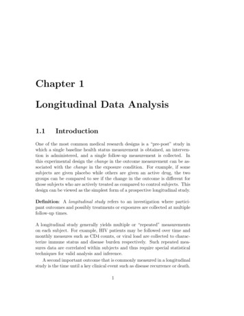
Linear Models for Quantitative ResponseNotation:yit is the value of the response variable for individual i at time t.zi is a column vector of variables that describe individuals but do not varyover timexit is a column vector of variables that vary both over individuals and overtimeBasic model:yit μt βxit γzi ε it ,i 1, , n ; t 1, ,Twhere ε is a random error term with mean 0 and constant variance, assumed tobe uncorrelated with x and z.β and γ are row vectors of coefficients.No lags, different intercepts at each time point, coefficients the same at alltime points.Consider OLS (ordinary least squares) estimation. Coefficients will be unbiased but not efficient. An efficient estimator isone whose true standard error is as small as possible, i.e., minimalvariability across repeated samples. Estimated standard errors will be too low because corr(εit, εit’) 0Example:581 children interviewed in 1990, 1992, and 1994 as part of the NationalLongitudinal Survey of Youth (NLSY).Copyright 2018 by Paul D. Allison7

Time-varying variables:ANTIantisocial behavior, measured with a scale ranging from 0 to 6.SELFself-esteem, measured with a scale ranging from 6 to 24.POVpoverty status of family, coded 1 for in poverty, otherwise 0.Time-invariant variables:BLACK1 if child is black, otherwise 0HISPANIC1 if child is Hispanic, otherwise 0CHILDAGEchild’s age in 1990MARRIED1 if mother was currently married in 1990, otherwise 0GENDER1 if female, 0 if maleMOMAGEmother’s age at birth of childMOMWORK1 if mother was employed in 1990, otherwise 0Original data set nlsy.dta has 581 records, one for each child, with differentnames for the variables at each time point, e.g., ANTI90, ANTI92 andANTI94.Before converting from the wide form to the long form, let’s look at the overtime correlations for the dependent variable.use c:\data\nlsy.dta, clearcorr anti*Copyright 2018 by Paul D. Allison8

(obs 581) anti90anti92anti94------------- --------------------------anti90 1.0000anti92 0.63801.0000anti94 0.54470.60081.0000Note that the 4-year lag correlation is smaller than the two 2-year lagcorrelations.Using the reshape command, we now convert the data into the long form, aset of 1743 records, one for each child in each year:use c:\data\nlsy.dta, cleargen id nreshape long anti self pov, i(id) j(year)save persyr3, replaceDatawide- ----------Number of obs.581- 1743Number of variables17- 12j variable (3 values)- yearxij variables:anti90 anti92 anti94- antiself90 self92 self94- selfpov90 pov92 pov94- ----------Note:The time-invariant variables are repeated across the multiple records foreach child.The variable id has a unique ID number for each child.Copyright 2018 by Paul D. Allison9

The variable year has values of 90, 92 or 94.Now we’ll do OLS regression, with no correction for dependencereg anti self pov black hispanic childage marriedgender momage momwork i.yearSource SSdfMS------------- -----------------------------Model 380.8578911 34.6234446Residual 3952.25743 1731 2.28322208------------- -----------------------------Total 4333.11532 1742 2.48743704Number of obsF( 11, 1731)Prob FR-squaredAdj R-squaredRoot MSE ---------anti Coef.Std. Err.tP t [95% Conf. Interval]------------- -------------self -.0741425.0109632-6.760.000-.095645-.0526401pov .4354025.08552755.090.000.2676544.6031505black .1678622.08818391.900.057-.0050959.3408204hispanic age .087056.06221211.400.162-.0349628.2090747married -.0888875.087227-1.020.308-.2599689.082194gender -.4950259.0728886-6.790.000-.637985-.3520668momage k .2120961.08000712.650.008.0551754.3690168year 92 .0521538.08871380.590.557-.1218437.226151294 .2255775.08886392.540.011.0512856.3998694cons Although the coefficients are unbiased, they are not efficient (truestandard errors are larger than necessary).More important, reported standard errors and p-values are probably toolowCopyright 2018 by Paul D. Allison10

Solution 1: Robust standard errorsRobust standard errors are standard error estimates that correct for dependenceamong the repeated observations. Also known as Huber-White standard errors,sandwich estimates, or empirical standard errors.For OLS linear models, conventional standard errors are obtained by firstcalculating the estimated covariance matrix of the coefficient estimates:s 2 (X' X ) 1where s2 is the residual variance and X is a matrix of dimension Tn K (n isthe number of individuals, T is the number ot time periods, and K is thenumber of coefficients). Standard errors are obtained by taking the squareroots of the main diagonal elements of this matrix.The formula for the robust covariance estimator isˆ ( X ' X ) 1 X′ y X βˆ y X βˆ ′ X ( X ' X ) 1Viiiiii i ()()where Xi is a T x K matrix of covariate values for individual i and yiis a T x 1 vector of y values for individual i. The robust standard errors are thesquare roots of the main diagonal elements of V̂ .In Stata, this method can be implemented with most regression commandsusing the vce option:reg anti self pov black hispanic childage marriedmomage gender momwork i.year, vce(cluster id)Linear regressionNumber of obs F( 11,580) Prob F Copyright 2018 by Paul D. Allison17438.990.000011