Transcription
Chapter 1Longitudinal Data Analysis1.1IntroductionOne of the most common medical research designs is a “pre-post” study inwhich a single baseline health status measurement is obtained, an intervention is administered, and a single follow-up measurement is collected. Inthis experimental design the change in the outcome measurement can be associated with the change in the exposure condition. For example, if somesubjects are given placebo while others are given an active drug, the twogroups can be compared to see if the change in the outcome is different forthose subjects who are actively treated as compared to control subjects. Thisdesign can be viewed as the simplest form of a prospective longitudinal study.Definition: A longitudinal study refers to an investigation where participant outcomes and possibly treatments or exposures are collected at multiplefollow-up times.A longitudinal study generally yields multiple or “repeated” measurementson each subject. For example, HIV patients may be followed over time andmonthly measures such as CD4 counts, or viral load are collected to characterize immune status and disease burden respectively. Such repeated measures data are correlated within subjects and thus require special statisticaltechniques for valid analysis and inference.A second important outcome that is commonly measured in a longitudinalstudy is the time until a key clinical event such as disease recurrence or death.1
2CHAPTER 1.LONGITUDINAL DATA ANALYSISAnalysis of event time endpoints is the focus of survival analysis which iscovered in chapter ?.Longitudinal studies play a key role in epidemiology, clinical research, andtherapeutic evaluation. Longitudinal studies are used to characterize normalgrowth and aging, to assess the effect of risk factors on human health, andto evaluate the effectiveness of treatments.Longitudinal studies involve a great deal of effort but offer several benefits. These benefits include:Benefits of longitudinal studies:1. Incident events are recorded. A prospective longitudinal study measures the new occurance of disease. The timing of disease onset can becorrelated with recent changes in patient exposure and/or with chronicexposure.2. Prospective ascertainment of exposure. In a prospective study participants can have their exposure status recorded at multiple follow-upvisits. This can alleviate recall bias where subjects who subsequentlyexperience disease are more likely to recall their exposure (a form ofmeasurement error). In addition the temporal order of exposures andoutcomes is observed.3. Measurement of individual change in outcomes. A key strength of alongitudinal study is the ability to measure change in outcomes and/orexposure at the individual level. Longitudinal studies provide the opportunity to observe individual patterns of change.4. Separation of time effects: Cohort, Period, Age. When studying changeover time there are many time scales to consider. The cohort scale isthe time of birth such as 1945 or 1963, period is the current time suchas 2003, and age is (period - cohort), for example 58 2003-1945,and 40 2003-1963. A longitudinal study with measurements at timest1 , t2 , . . . tn can simultaneously characterize multiple time scales such asage and cohort effects using covariates derived from the calendar timeof visit and the participant’s birth year: the age of subject i at timetj is ageij (tj birthi ); and their cohort is simply cohortij birthi .Lebowitz [1996] discusses age, period, and cohort effects in the analysisof pulmonary function data.
1.1.INTRODUCTION35. Control for cohort effects. In a cross-sectional study the comparisonof subgroups of different ages combines the effects of aging and theeffects of different cohorts. That is, comparison of outcomes measuredin 2003 among 58 year old subjects and among 40 year old subjectsreflects both the fact that the groups differ by 18 years (aging) andthe fact that the subjects were born in different eras. For example, thepublic health interventions such as vaccinations available for a childunder 10 years of age may difer during 1945-1955 as compared to thepreventive interventions experienced in 1963-1973. In a longitudinalstudy the cohort under study is fixed and thus changes in time are notconfounded by cohort differences.An overview of longitudinal data analysis opportunities in respiratory epidemiology is presented in Weiss and Ware [1996].The benefits of a longitudinal design are not without cost. There areseveral challenges posed:Challenges of longitudinal studies:1. Participant follow-up. There is the risk of bias due to incomplete followup, or “drop-out” of study participants. If subjects that are followed tothe planned end of study differ from subjects who discontinue follow-upthen a naive analysis may provide summaries that are not representative of the original target population.2. Analysis of correlated data. Statistical analysis of longitudinal datarequires methods that can properly account for the intra-subject correlation of response measurements. If such correlation is ignored theninferences such as statistical tests or confidence intervals can be grosslyinvalid.3. Time-varying covariates. Although longitudinal designs offer the opportunity to associate changes in exposure with changes in the outcomeof interest, the direction of causality can be complicated by “feedback”between the outcome and the exposure. For example, in an observational study of the effects of a drug on specific indicators of health,a patient’s current health status may influence the drug exposure ordosage received in the future. Although scientific interest lies in theeffect of medication on health, this example has reciprocal influence
4CHAPTER 1.LONGITUDINAL DATA ANALYSISbetween exposure and outcome and poses analytical difficulty whentrying to separate the effect of medication on health from the effect ofhealth on drug exposure.1.1.1ExamplesIn this subsection we give some examples of longitudinal studies and focus onthe primary scientific motivation in addition to key outcome and covariatemeasurements.(1.1) Child Asthma Management Program (CAMP) – In this studychildren are randomized to different asthma management regimes. CAMP isa multicenter clinical trial whose primary aim is the evaluation of the longterm effects of daily inhaled anti-inflammatory medication use on asthmastatus and lung growth in children with mild to moderate ashtma (Szefleret al. 2000). Outcomes include continuous measures of pulmonary functionand catergorical indicators of asthma symptoms. Secondary analyses haveinvestigated the association between daily measures of ambient pollution andthe prevalence of symptoms. Analysis of an environmental exposure requiresspecification of a lag between the day of exposure and the resulting effect.In the air pollution literature short lags of 0 to 2 days are commonly used(Samet et al. 2000; Yu et al. 2000). For both the evaluation of treatmentand exposure to environmental pollution the scientific questions focus on theassociation between an exposure (treatment, pollution) and health measures.The within-subject correlation of outcomes is of secondary interest, but mustbe acknowledged to obtain valid statistical inference.(1.2) Cystic Fibrosis and Pulmonary Function – The Cystic Fibrosis Foundation maintains a registry of longitudinal data for subjects withcystic fibrosis. Pulmonary function measures such as the 1-second forcedexpiratory volume (FEV1) and patient health indicators such as infectionwith Pseudomonas aeruginosa have been recorded annually since 1966. Onescientific objective is to characterize the natural course of the disease andto estimate the average rate of decline in pulmonary function. Risk factoranalysis seeks to determine whether measured patient characteristics such asgender and genotype correlate with disease progression, or with an increasedrate of decline in FEV1. The registry data represent a typical observationaldesign where the longitudinal nature of the data are important for determin-
1.1.INTRODUCTION5ing individual patterns of change in health outcomes such as lung function.(1.3) The Multi-Center AIDS Cohort Study (MACS) – The MACSstudy enrolled more than 3,000 men who were at risk for acquisition of HIV1(Kaslow et al. 1987). This prospective cohort study observed N 479 incident HIV1 infections and has been used to characterize the biological changesassociated with disease onset. In particular, this study has demonstrated theeffect of HIV1 infection on indicators of immunologic function such as CD4cell counts. One scientific question is whether baseline characteristics suchas viral load measured immediately after seroconversion are associated witha poor patient prognosis as indicated by a greater rate of decline in CD4 cellcounts. We use these data to illustrate analysis approaches for continuouslongitudinal response data.(1.4) HIVNET Informed Consent Substudy – Numerous reports suggest that the process of obtaining informed consent in order to participate inresearch studies is often inadequate. Therefore, for preventive HIV vaccinetrials a prototype informed consent process was evaluated among N 4, 892subjects participating in the Vaccine Preparedness Study (VPS). Approximately 20% of subjects were selected at random and asked to participate in amock informed consent process (Coletti et al. 2003). Participant knowledgeof key vaccine trial concepts was evalulated at baseline prior to the informedconsent visit which occured during a special 3 month follow-up visit for theintervention subjects. Vaccine trial knowledge was then assessed for all participants at the scheduled 6, 12, and 18 month visits. This study design isa basic longitudinal extension of a pre-post design. The primary outcomesinclude individual knowledge items, and a total score that calculates thenumber of correct responses minus the number of incorrect responses. Weuse data on a subset of men and women VPS participants. We focus onsubjects who were considered at high risk of HIV acquisition due to injectiondrug use.1.1.2NotationIn this chapter we use Yij to denote the outcome measured on subject i at timetij . The index i 1, 2, . . . , N is for subject, and the index j 1, 2, . . . , nis for observations within a subject. In a designed longitudinal study themeasurement times will follow a protocol with a common set of follow-up
6CHAPTER 1.LONGITUDINAL DATA ANALYSIStimes, tij tj . For example, in the HIVNET Informed Consent Study subjects were measured at baseline, t1 0, at 6 months after enrollment, t2 6months, and at 12 and 18 months, t3 12 months, t4 18 months. We letXij denote covariates associated with observation Yij . Common covariatesin a longitudinal study include the time, tij , and person-level characteristicssuch as treatment assignment, or demographic characteristics.Although scientific interest often focuses on the mean response as a function of covariates such as treatment and time, proper statistical inferencemust account for the within-person correlation of observations. Define ρjk corr(Yij , Yik ), the within-subject correlation between observations at times tjand tk . In the following section we discuss methods for explorating the structure of within-subject correlation, and in section 1.5 we discuss estimationmethods that model correlation patterns.1.2Exploratory Data AnalysisExploratory analysis of longitudinal data seeks to discover patterns of systematic variation across groups of patients, as well as aspects of randomvariation that distinguish individual patients.1.2.1Group means over timeWhen scientific interest is in the average response over time, summary statistics such as means and standard deviations can reveal whether differentgroups are changing in a similar or different fashion.Example 1 Figure 1.1 shows the mean knowledge score for the informedconsent subgroups in the HIVNET Informed Consent Substudy. At baselinethe intervention and control groups have very similar mean scores. This isexpected since the group assignment is determined by randomization whichoccurs after enrollment. At an interim 3 month visit the intervention subjects are given a mock informed consent for participation in a hypotheticalphase III vaccine efficacy trial. The impact of the intervention can be seenby the mean scores at the 6 month visit. In the control group the meanat 6 months is 1.49 (S.E. 0.11), up slightly from the baseline mean of 1.16(S.E. 0.11). In contrast, the intervention group has a 6 month mean score of
1.2.7EXPLORATORY DATA ANALYSIS3.43 (S.E. 0.24), a large increase from the baseline mean of 1.09 (S.E. 0.24).The intervention and control groups are significantly different at 6 montsbased on a 2-sample t-test. At later follow-up times further change is observed. The control group has a mean that increases to 1.98 at the 12 monthvisit and to 2.47 at the 18 month visit. The intervention group fluctuatesslightly with means of 3.25 (S.E. 0.27) at month 12, and 3.76 (S.E. 0.25) at18 months. These summaries suggest that the intervention has a significanteffect on knowledge, and that small improvement is seen over time in thecontrol group.6Vaccine Figure 1.1: Mean knowledge scores over time by treatment group, HIVNETInformed Consent Substudy.
8CHAPTER 1.LONGITUDINAL DATA ANALYSISExample 2 In the MACS study we compare different groups of subjectsformed on the basis of their initial viral load measurement. Low viral load isdefined by a baseline value less than 15 103 , medium as 15 103 - 46 103 ,and high viral load is classified for subjects with a baseline measurementgreater than 46 103 . Table 1.1 gives the average CD4 count for each year offollow-up. The mean CD4 declines over time for each of the viral load groups.Table 1.1: Mean CD4 count and standard error over time. Separate summaries are given for groups defined by baseline viral load level.year0-11-22-33-4Lowmean (S.E.)744.8 (35.8)721.2 (36.4)645.5 (37.7)604.8 (46.8)Baseline Viral LoadMediummean (S.E.)638.9 (27.3)588.1 (25.7)512.8 (28.5)470.0 (28.7)Highmean (S.E.)600.3 (30.4)511.8 (22.5)474.6 (34.2)353.9 (28.1)The subjects with the lowest baseline viral load have a mean of 744.8 for thefirst year after seroconversion and then decline to a mean count of 604.8 during the fourth year. The 744.8-604.8 140.0 unit reduction is smaller thanthe decline observed for the medium viral load group, 638.9-470.0 168.9,and the high viral load group, 600.3-353.9 246.4. Therefore, these summaries suggest that higher baseline viral load measurements are associatedwith greater subsequent reduction in mean CD4 counts.Example 3 In the HIVNET Informed Consent Substudy we saw a substantial improvement in the knowledge score. It is also relevent to consider keyindividual items that comprise the total score such as the “safety item” orthe “nurse item.” Regarding safety, participants were asked whether it wastrue or false that “Once a large-scale HIV vaccine study begins, we can besure the vaccine is completely safe.” Table 1.2 shows the number of responding subjects at each visit and the percent of subjects who correctly answeredthat the safety statement is false. These data show that the control andintervention groups have a comparable understanding of the safety item at
1.2.9EXPLORATORY DATA ANALYSISTable 1.2: Number of subjects and percent answering correctly for the safetyitem from the HIVNET Informed Consent Substudy.visitbaseline6 month12 month18 monthControl GroupN % correct94640.983842.780941.578243.5Intervention GroupN% correct17639.217150.316343.615343.1baseline with 40.9% answering correctly among controls, and 39.2% answering correctly among the intervention subjects. A mock informed consentwas administered at a 3 month visit for the intervention subjects only. Theimpact of the intervention appears modest with only 50.3% of interventionsubjects correctly responding at 6 months. This represents a 10.9% increasein the proportion answering correctly, but a 2-sample comparison of intervention and control proportions at 6 months (eg. 50.3% versus 42.7%) is notstatistically significant. Finally, the modest intervention impact does not appear to be retained as the fraction correctly answering this item declines to43.6% at 12 months and 43.1% at 18 months. Therefore, these data suggesta small but fleeting improvement in participant understanding that a vaccinestudied in a phase III trial can not be guaranteed to be safe.Other items show different longitudinal trends. Subjects were also askedwhether it was true or false that “The study nurse will decide who gets thereal vaccine and who gets the placebo.” Table 1.3 shows that the groupsare again comparable at baseline, but for the nurse item we see a largeincrease in the fraction answering correctly among intervention subjects at6 months with 72.1% correctly answering that the statement is false. Across-sectional analysis indicates a statistically significant difference in theproportion answering correctly at 6 months with a confidence interval forthe difference in proportions of (0.199, 0.349). Although the magnitude of theseparation between groups decreases from 27.4% at 6 months to 17.8% at 18months, the confidence interval for the difference in proportions at 18 monthsis (0.096, 0.260) and excludes the null comparison, p1 p0 0. Therefore,these data suggest that the intervention has a substantial and lasting impacton understanding that research nurses do not determine allocation to real
10CHAPTER 1.LONGITUDINAL DATA ANALYSISTable 1.3: Number of subjects and percent answering correctly for the nurseitem from the HIVNET Informed Consent Substudy.visitbaseline6 month12 month18 monthControl GroupN % correct94554.183844.780846.378248.2Intervention GroupN% correct17650.317172.116360.115366.0vaccine or placebo.1.2.2Variation among individualsWith independent observations we can summarize the uncertainty or variablibility in a response measurement using a single variance parameter. Oneinterpretation of the variance is given as one half the expected squared distance between any two randomly selected measurements, σ 2 21 E[(Yi Yj )2 ].However, with longitudinal data the “distance” between measurements ondifferent subjects is usually expected to be greater than the distance betweeen repeated measurements taken on the same subject. Thus, althoughthe total variance may be obtained with outcomes from subjects i and i0 observed at time tj , σ 2 21 E[(Yij Yi0 j )2 ] (assuming that E(Yij ) E(Yi0 j ) µ),the expected variation for two measurements taken on the same person (subject i) but at times tj and tk may not equal the total variation σ 2 since themeasurements are correlated: σ 2 (1 ρjk ) 21 E[(Yij Yik )2 ] (assuming thatE(Yij ) E(Yik ) µ). When ρjk 0 this shows that between-subject variation is greater than within-subject variation. In the extreme ρjk 1 andYij Yik implying no variation for repeated observations taken on the samesubject.Graphical methods can be used to explore the magnitude of person-toperson variability in outcomes over time. One approach is to create a panelof individual line plots for each study participant. These plots can then beinspected for both the amount of variation from subject-to-subject in theoverall “level” of the response, and the magnitude of variation in the “trend”over time in the response. Such exploratory data analysis can be useful for
1.2.EXPLORATORY DATA ANALYSIS11determining the types of correlated data regression models that would beappropriate. Section 1.5 discusses random effects regression models for longitudinal data. In addition to plotting individual series it is also useful toplot multiple series on a single plot stratifying on the value of key covariates.Such a plot allows determination whether the type and magnitude of intersubject variation appears to differ across the covariate subgroups.Example 4 In Figure 1.2 we plot an array of individual series from theMACS data. In each panel the observed CD4 count for a single subject isplotted against the times that measurements were obtained. Such plots allowinspection of the individual response patterns and whether there is strongheterogeneity in the trajectories. Figure 1.2 shows that there can be largevariation in the “level” of CD4 for subjects. Subject ID 1120 in the upperright corner has CD4 counts greater than 1000 for all times while ID 1235 inthe lower left corner has all measurements below 500. In addition, individualsplots can be evaluated for the change over time. Figure 1.2 indicates thatmost subjects are either relatively stable in their measurements over time, ortend to be decreasing.In the common situation where we are interested in correlating the outcome to measured factors such as treatment group or exposure it will also beuseful to plot individual series stratified by covariate group. Figure 1.3 takesa sample of the MACS data and plots lines for each subject stratified by thelevel of baseline viral load. This figure suggests that the highest viral loadgroup has the lowest mean CD4 count, and suggests that variation amongmeasurements may also be lower for the high baseline viral load group ascompared to the medium and low groups. Figure 1.3 can also be used toidentify individuals who exhibit time trends that differ markedly from otherindividuals. In the high viral load group there is an individual that appears todramatically improve over time, and there is a single unusual measurementwhere the CD4 count exceeds 2000. Plotting individual series is a usefulexploratory prelude to more careful confirmatory statistical analysis.1.2.3Characterizing correlation and covarianceWith correlated outcomes it is useful to understand the strength of correlation and the pattern of correlations across time. Characterizing correlation
12CHAPTER 1.101505203040LONGITUDINAL DATA re 1.2: A sample of individual CD4 trajectories from the MACS data.is useful for understanding components of variation and for identifying avariance or correlation model for regression methods such as mixed-effectsmodels or generalized estimating equations (GEE) discussed in section 1.5.2.One summary that is used is an estimate of the covariance matrix which isdefined as: E[(Yi1 µi1 )2 ]E[(Yi1 µi1 )(Yi2 µi2 )] . . . E[(Yi1 µi1 )(Yin µin )] E[(Yi2 µi2 )(Yi1 µi1 )]E[(Yi2 µi2 )2 ]. . . E[(Yi2 µi2 )(Yin µin )] . .E[(Yin µin )(Yi1 µi1 )] E[(Yin µin )(Yi2 µi2 )] . . .E[(Yin µin )2 ] .
1.2.EXPLORATORY DATA ANALYSIS13The covariance can also be written in terms of the variances σj2 and thecorrelations ρjk : σ12σ1 σ2 ρ12 . . . σ1 σn ρ1n σ2 σ1 ρ21σ22. . . σ2 σn ρ2n cov(Yi ) . .2σn σ1 ρn1 σn σ2 ρn2 . . .σnFinally, the correlation matrix is given as 1 ρ12 . . . ρ1n ρ21 1 . . . ρ2n corr(Yi ) . . . . ρn1 ρ2n . . . 1which is useful for comparing the strength of association between pairs of outcomes particularly when the variances σj2 are not constant. Sample estimatesof the correlations can be obtained usingρbjk 1 X (Yij Y ·j ) (Yik Y ·k )N 1 iσbjσbkwhere σbj2 and σbk2 are the sample variances of Yij and Yik respectively, i.e.across subjects for times tj and tk .Graphically the correlation can be viewed using plots of Yij versus Yikfor all possible pairs of times tj and tk . These plots can be arranged in anarray that corresponds to the covariance matrix and patterns of associationacross rows or columns can reveal changes in the correlation as a function ofincreasing time separation between measurements.Example 5 For the HIVNET informed consent data we focus on correlation analysis of outcomes from the control group. Parallel summaries wouldusefully characterize the similarity or difference in correlation structures forthe control and intervention groups. The correlation matrix is estimated as:monthmonthmonthmonth061218month 0 month 6 month 12 month 1.000.5080.3130.4070.5081.00
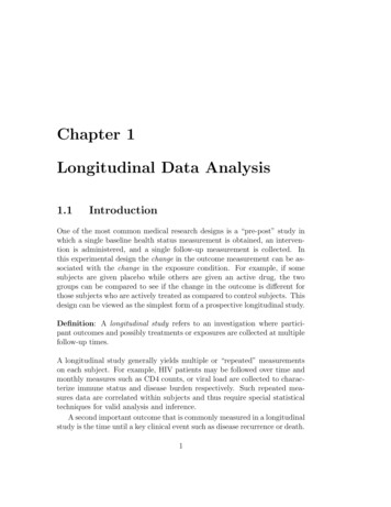
14CHAPTER 1.LONGITUDINAL DATA ANALYSISThe matrix suggests that the correlation in outcomes from the same individual is slightly decreasing as the time between the measurements increases.For example, the correlation between knowledge scores from baseline andmonth 6 is 0.471, while the correlation between baseline and month 12 decreases to 0.394, and further decreases to 0.313 for baseline and month 18.Correlation that decreases as a function of time separation is common amongbiomedical measurements and often reflects slowly varying underlying processes.Example 6 For the MACS data the timing of measurement is only approximately regular. The following displays both the correlation matrix and thecovariance matrix:year 1year 2year 3year 4year 1 92280.4 [ 0.734] [ 0.585][ 0.574]year 2 63589.4 81370.0 [ 0.733][ 0.695]year 3 48798.2 57457.5 75454.5[ 0.806]year 4 55501.2 63149.9 70510.1 101418.2In brackets above the diagonal are the correlations. On the diagonal are thevariances.For example, the standard deviation among year 1 CD4 counts is 92280.4 303.8, while the standard deviations for years 2 through 4 are 81370.0 2853, 75454.5 274.7, and 101418.2 318.5 respectively.Below the diagonal are the covariances which together with the standard deviations determine the correlations. These data have correlation for measurements that are one year apart of 0.734, 0.733 and 0.806. For measurementstwo years apart the correlation decreases slightly to 0.585 and 0.695. Finally,measurements that are three years apart have a correlation of 0.574. Thus,the CD4 counts have a within-person correlation that is high for observationsclose together in time, but the correlation tends to decrease with increasingtime separation between the measurement times.An alternative method for exploring the correlation structure is throughan array of scatter plots showing CD4 measured at year j versus CD4 measured at year k. Figure 1.4 displays these scatter plots. It appears that thecorrelation in the plot of year 1 versus year 2 is stronger than for year 1 versus year 3, or for year 1 versus year 4. The sample correlations ρb12 0.734,ρb13 0.585, and ρb14 0.574 summarize the linear association presented inthese plots.
1.2.15EXPLORATORY DATA ANALYSIS10Low Viral Load203040Medium Viral LoadHigh Viral Load2000cd41500100050001020304010203040monthFigure 1.3: Individual CD4 trajectories from the MACS data by tertile ofviral load.
14000 year 120060010001400 year 2 150010005000 1000 1500 year 3 1000 500 5001500 1000 500 1500 100010005006001500200LONGITUDINAL DATA ANALYSIS1000CHAPTER 1.50016year 41500Figure 1.4: Scatterplots of CD4 measurements (counts/ml) taken at years1-4 after seroconversion.
1.3.DERIVED VARIABLE ANALYSIS1.317Derived Variable AnalysisFormal statistical inference with longitudinal data requires either that a univariate summary be created for each subject or that methods for correlateddata are used. In this section we review and critique common analytic approaches based on creation of summary measures. A derived variable analysisrefers to a method that takes a collection of me
6 CHAPTER 1. LONGITUDINAL DATA ANALYSIS times, tij tj.For example, in the HIVNET Informed Consent Study sub-jects were measured at baseline, t1 0, at 6 months after enrollment, t2 6 months, and at 12 and 18 months, t3 12 months, t4 18 months. We let