WIXLIB

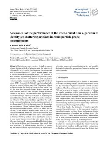
C. Proposed Method 2: Two-Layer Nonlinear NeuralNetwork EstimatorThis approach is to calculate the weight ! of EWMA dynamically according to the traffic behaviour, then combine it with EWMA method to estimate inter-arrival time.We use two-layer nonlinear neural network model forobtaining the weight ! of EWMA.The model is illustrated in the same figure as Figure 1with y replaced by ! , i.e., ! f (r ) , where f is a nonlinear sigmoid function defined asf (1 e ! r ) !1 with0 ! f 1 . As described in Method 1 above, the observed traffic histories are used for input samples. Thesamples are updated by the most recent data. In thismodel the weight ! is varied between 0 and 1 due to thetraffic status.The training is based on a gradient descent in errorspace in the same way as Method 1. Because sigmoidfunction is nonlinear we can not calculate learning ratedirectly like in Method 1. A simple method of effectivelyincreasing the learning speed is to modify the delta ruleby including a momentum term [9]. The adjusted valuesof weights and threshold are defined as:"wi (t ) % (u ! x[k ])( x[k ! 1] ! x[k ! 1])(1 ! ) xi!!!!! #"wi (t ! 1) !!!i 1,., n"# (t ) & (u ! x[k ])( x[k ! 1] ! x[k ! 1])(1 ! % )%!!!!! "# (t ! 1)where λ is a positive constant which is determined experimentally. The learning rate η in the method is a positive constant as well.D. Proposed Method 3: Multi-Layer Neural NetworkEstimatorIn this method, a three-layer neural network with backpropagation algorithm is applied to inter-arrival time estimation. It consists of an input layer with n neurons, onehidden layer with m neurons, and an output layer with oneneuron. Figure 2 illustrates the structure of the neuralnetwork. The sigmoid transfer function is utilized to generate the output of each neuron from its compound inputs.The output of each neuron is connected to the input of allthe neurons in the succeeding layer after being multipliedby the weights.The observed inter-arrival time samples are input tothe first layer then we obtain the estimated value from theoutput layer. The training algorithm is based on backpropagation algorithm [9]. It propagates the output errorto the preceding layer via the existing connections untilthe input layer. The neural model also has a bias term ininput and hidden layers, but in the following explanation,it is abbreviated for simplicity.We use the following notation for explaining the learning algorithm. x1.xn are the input samples and used as the firstlayer inputs.y1. ym indicate the outputs of the hidden layer z represents an output of the networkvij denotes a weight of the connection between jth neuron from input layer and the ith neuron of hiddenlayerwi denotes a weight of the connection between ith neuron from hidden layer and a neuron of outputlayerThus,nri ! vij x j , yi f (ri ) , i 1,., mj 1ms ! wi yi ,z f (s )i 1where f is the sigmoid function.The adjustment is calculated with leaning rate andmomentum term. Weight adjustments are defined as"vij (t ) % {(u ! z ) f #( s ) wi . f #(ri ) x j } "vij (t ! 1)"wi (t ) % {(u ! z ) f #( s ) yi } "wi (t ! 1)f " f (1 ! f )The input inter-arrival times are normalized within therange [0.1, 0.9] before being passed to the neural network[10]. The estimated value from neural network is denormalized.X normalized X denormalizedX input ! X min( HI ! LO ) LOX max ! X minX! LO output( X max ! X min ) X minHI ! LOwhere Xinput is input value, Xmin and Xmax are the minimumand maximum of observed inter-arrival times respectively.Xoutput is an output of the neural network. HI and LI are setto 0.1 and 0.9 respectively.x1y1x2y2xn!1ym!1ymxnInput LayerHidden LayerzOutput LayerFigure 2 Three-layer neural network.

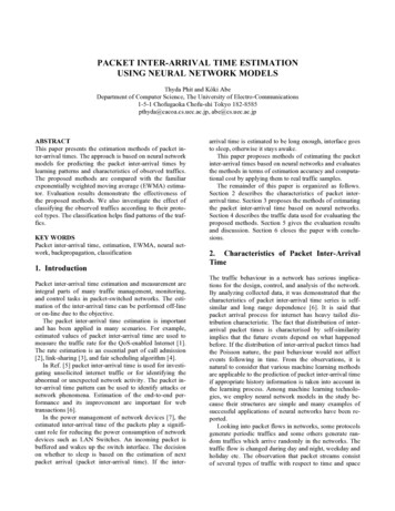
4. Traffic Data Used for Evaluation%"#Internet%234015116789:;6.0 To evaluate the methods proposed above, the traffic datacollected at a real network is used, the topology of whichis shown in Figure 3 [7]. The traffic data was measuredfor 2 hours on a regular workday by tcpdump for gathering traces and then the traces were analyzed using theethereal tool. The entire traffic consists of different protocol traffics. They are IP protocol traffic (which consists ofCDP, RPC1, ICMP, and OSPF2), STP3, CDP4, and others.We used the traffics of two different connections, one is aconnection between Switch FA to Host Y called Host Yand the other is a connection between Switch FA toSwitch FB called Switch FB. "# !"#! % & ' # ( ) * ! % & ' # ( ) * Figure 4 Inter-arrival time ,-./01distribution of unclassifiedtraffics of Host Y: 200 packets from the beginning.%"#LAN5router Nrouter PLAN 6stp root switch5LAN 3HostYswitch FA .switch FB .LAN 4234015116789: ;6.0 switch F20% . .LAN 1 "# !"#LAN2Figure 3 Network topology.! Type 01421IPTable 1 Traffic data of Host Y.Type 1Type 2Type 35657186371STPCDPOthersTotal7635Table 1 shows the collected traffic of Host Y to SwitchFA connection during light activity time which was usedin our evaluation. The traffic data was classified intotypes 0, 1, 2 and 3 which denote IP, STP, CDP, and otherstraffics, respectively.Figure 4 illustrates a starting part of distribution of unclassified traffics of Host Y. In the figure, the horizontalaxis is the arrival packet sequence number while the vertical axis is an inter-arrival time of the traffics. The interarrival time varies from 0 to 2.5 second. Some protocolsgenerate periodic traffics like at number 11, 31 and so on.The entire traffic has similar patterns to the segmentshown in the figure.Type 2 traffic data of Host Y, as shown in Figure 5, isfound to be characterized as repetition of sub-patterns. Itappears to consist of several periodic traffics with different phases which are generated by CDP protocol of different devices.1Remote Procedure CallOpen Shortest Path First3Spanning-Tree Protocol4Cisco Discovery Protocol2 % & ' # ( ) * ! % & ' # ( ) * ,-./01Figure 5 Inter-arrival time distributionof traffic Type 2 ofHost Y.Table 2 Traffic data of Switch FB.Type 0Type 4Total99802010000IPARPTable 2 shows the collected traffic of Switch FB connection during light activity time which is also used in ourevaluation. We took 10000 traffics from colleted datathen classified into Type 0 and 4 which denote IP andARP packet protocol, respectively.Figure 6 illustrates the distribution of Switch FB traffics. 200 traffics are plotted from the traffic number 1000.There are many packets with inter-arrival times rangingfrom 0.35 to 0.45 millisecond which belong to trafficsgenerated by RPC protocol due to NFS (Network FileService) transactions.Type 0 traffics of Host Y and Switch FB consist of IPpackets generated by UDP, TCP, ICMP and OSPF protocols. Table 3 shows the percentages of those constituents.The UDP traffics of Switch FB mainly come from RPCprocedure calls.

5.1 Estimation Accuracy of Proposed Methods!"(!"' Figure 7 shows the average of relative estimation errorson the whole traffic data with different types. Method 3performs the best estimation except for Type 0 whichconsists of various kinds of packets including TCP, UDP,ICMP, and OSPF. The estimation accuracy for Type 0traffic would increase if the packets are classified morefinely.!"& !"&!" !" !"% !"%100!"# ))*())(!))(*))& ))'))) #))%%))# )))')) &))!()!*!)!**)!())!' )!&#)!% )! %)!#&)!)()! ')!!!)!!*!"#,-./01Figure 6 Inter-arrival time distribution of unclassifiedtraffics of Switch FB.Table 3 Constituents of Type 0 traffics.Host Y [%]Switch FB 40OSPF00.2990EWMA80Method 1Method 270Method 36050403020100T ype05. Evaluation Results and DiscussionsWe evaluate the proposed methods of inter-arrival timeestimation by applying them to the traffic described in theprevious section. We examine the effect of traffic classification as well. The estimation methods were implementedin C language and executed on a Linux machine of AMDAthlon 64 3000 operated at 2GHz with 2 GB mainmemory.The methods were evaluated in terms of relative errorof estimated time that is defined as below.relative error Average of Relative Estimation Errors (%)234015116789:;6.0 . !"' real " estimated ! 100[%]realThe parameters of the methods were determined experimentally so that the average of relative errors beminimum as shown in Table 4.T ype1T ype2T ype4Figure 7 Average of relative estimation errors of classified traffic.The detail of the estimation results compared with theobserved traffics is shown in Figure 8, taking the Type 2traffic data as an example. It illustrates a segment of traffics estimated by EWMA, Methods 1, 2 and 3. Figure 9plots their relative errors of estimation. According to thefigures, it is found that Method 3 yields the most accurateestimation of inter-arrival time among four estimators.The estimation accuracy of EWMA and Method 2were poor; they can not catch the characteristics of theobserved traffics. Method 1 can follow the behaviour ofthe observed traffic except the starting part of the segmentwhere the effect of the previous segment deteriorated theestimation accuracy. Method 3 has good performanceover all the segment except the inter-arrival time of number 13 where the behaviour of the observed trafficchanges abruptly.%"#Table 4 Experimentally determined parameters.EWMAMethod1Method 2Method 3SwitchFBHost YType 0Type 1Type 2Type λ0.8n881320η0.05λ0.5Type 0 "# !"#8mTotal%234015116789:;6.0 Traffics83! %&'#?089:;18@@6A()BCD5* ! % & ' # ( ),-./01D04EFG: D04EFG:%D04EFG:&Figure 8 A segment of traffics Type 2 estimated byEWMA, Methods 1, 2 and 3 compared with the real one.

results in a good performance. It is considered that classification helps the estimators find distinct traffic patterns.#!!"*!"5.3 Static and Dynamic EWMA Methods)!"(!"'!"&!"%!" !"#!"!"# %&'(9 ?)* #!,-./01 05@;A8### 05@;A8 # #%#&#'#(#) 05@;A8%Figure 9 Relative errors of a segment of traffics Type 2estimated by EWMA, Methods 1, 2 and 3.Average of Relative Estimation Errors (%)2520EWMAMethod 1Method 2Method 3151050Figure 10 Average of relative estimation errors ofSwitch FB Type 0 traffics estimated by EWMA, Methods1, 2 and 3.The average of relative estimation errors of Switch FBType 0 traffics are plotted in Figure 10. From the figure,the overall accuracy of estimation errors is good, beingdifferent from the case of Host Y. This is attributed to thedifference between the behaviours of IP packets of HostY and Switch FB traffics. Type 0 IP traffics of Switch FBare dominated by UDP packets generated by RPC due toNFS transactions. As shown in Figure 6 the pattern ofinter-arrival time is characterized to be somewhat regular,containing a small number of packets with long interarrival times. On the other hand Type 0 IP traffics of HostY consist of various kinds of packets including TCP, UDP,ICMP, and OSPF. As described previously, the estimationaccuracy for Type 0 traffics of Host Y would increase ifthe packets are classified more finely. Method 3 is foundto give the lowest errors for estimating Switch FB Type 0traffics as the case for estimating Host Y traffics.5.2 Effectiveness of ClassificationFigure 11 shows the result of relative estimation errorsfor unclassified and classified traffics. The gray bars denote the averaged errors of estimation on unclassifiedtraffics while the black bars denote errors averaged overindividual estimation on classified traffics except Type 0.According to the figures, classifying the traffics alwaysMethod 2 is a dynamic version of EWMA where theweight ! is determined dynamically by a neural networkmodel. According to Figure 11, it is found that varyingthe weight gives more accurate prediction than conventional EWMA with constant ! . However as seen in Figure 5, Method 2 fails to follow the behaviour of the observed traffics. It is found from static EWMA thatincreasing the weight α leads to better imitating the variation of the observed traffic but with considerable delays,while decreasing the weight makes the prediction insensitive to the current change of observed traffics. Therefore,even if the weight is adjusted dynamically in its magnitude as done in Method 2, improvements of the estimationperformance are limited.Average of Relative Estimation Errors (%)2034567089:56.456; 8911;1: !"40Unclassied T raffic35Classified T raffic302520151050EWMAMethod 1Method 2Method 3Figure 11 Average of relative estimation errors of unclassified and classified traffics.5.4 Computational Complexity of EstimatorsThe time required for each method to estimate the trafficswas measured. The result is shown in Table 5. The measurement was carried out for each method on the unclassified traffic with 7636 packets. EWMA with less estimation accuracy takes less time than the others. Method 3which provides the most accurate prediction takes thelongest time among all the methods. Thus, there is atrade-off between estimation accuracy and computationaltime. For instance Method 3 can be employed for suchapplications that require accurate estimation for light traffics. (Note that Method 3 takes 15 ms to predict the timewhen the next packet arrives.)Table 5 Time of estimation of each method on the unclassified traffic with 7636 packets.EWMA0.03[s]Method 10.04[s]Method 20.17[s]Method 3116.18[s]

6. Conclusions and Future WorkIn this paper, we proposed neural network models forestimating packet inter-arrival time of packet-switchednetworks. The results show that the models realize moreaccurate estimation than conventional EWMA method.We also investigated the effectiveness of classifying traffic by protocol types and found that it helps estimatorsfind distinct traffic patterns, resulting in accurate estimation. The accuracy, however, is obtained at the cost ofcomputational complexity. The preferable method to beemployed for an application depends on whether it requires estimation accuracy or estimation time.We need to further evaluate the proposed methods byapplying them to the other traffics observed in the realnetwork shown in Figure 3.AcknowledgmentsWe would like to thank Dr. M. Gupta with ComputerScience Department of Portland State University forkindly providing us with the network traffic data collectedat a real network. We also would like to thank the anonymous reviewers for numerous suggestions improving thismanuscript. It was partially supported by JSPS Grant-inAid for Scientific Research (C) (2) 18500048.References[1] F. Agharebparast, and V. C. M. Leung, A new trafficrate estimation and monitoring algorithm for theQoS-enabled Internet, Global TelecommunicationsConference 2003(GLOBECOM '03.), vol. 7, pp.3883- 3887, Dec. 2003.[2] M. Grossglauser and D. Tse, A framework for robustmeasurement based admission control, IEEE/ACMTrans. Networking, vol. 7(3), pp.293-309, June 1999.[3] S. Floyd and V. Jacobson, Link-sharing and resourcemanagement models for packet networks,IEEE/ACM Trans. Networking, vol. 3 pp.365-386,Aug. 1995.[4] F. Agharebparast and V.C.M. Leung, Efficient fairqueuing with decoupled delay-bandwidth guarantees,in Proc. IEEE Globecom’01, San Antonio, TX,pp.2601-2605, Nov. 2001.[5] J. Zimmermann, A. Clacrk and G. Mohay, The use ofpacket inter-arrival times for investigating unsolicited internet traffic, Proc. The first InternationalWorkshop on Systematic Approaches to DigitalForensic Engineering (SADFE’05), pp. 89 - 104,Nov. 2005.[6] T. Kushida and Y. Shibata, Empirical study of interarrival packet times and packet losses, Proc. 22ndInternational Conference on Distributed ComputingSystems Workshops(ICDCSW’02), pp.233 - 238,July 2002.[7] M. Gupta, S. Glover, and S. Singh, A Feasibilitystudy for power management in LAN switches. Proc.12th IEEE International Conference on Network Protocols, pp. 361-371, Oct. 2004.[8] M. Minsky and S. Papert, Perceptrons, Cambridge,MA, The MIT Press, 1969.[9] S. Murray, Neural Networks for Statistical Modeling,Library of Congress Cataloging-in-Publication Data,1994.[10] Y. Sugai, Learning and Its Algorithms, Chapter 4 (inJapanese), Morikita Publishing Co., 2002.

Packet inter-arrival time, estimation, EWMA, neural net-work, backpropagation, classification 1. Introduction Packet inter-arrival time estimation and measurement are integral parts of many traffic management, monitoring, and control tasks in packet-switched networks. The esti-mation of the inter-arrival time can be performed off-line