WIXLIB

A. Korolev and P. R. Field: Assessment of the performance of the inter-arrival time algorithmFigure 1. Conceptual diagram of the distribution of inter-arrivaltimes φ(1t) with well separated short and long inter-arrival timemodes (a), when shattering artifacts can be segregated from the intact particles. When the distributions of inter-arrival time associatedwith intact particles φi (1t) and shattered fragments φs (1t) havesignificant overlap, then segregation of intact particles and shatteredartifacts is hindered (b).particles satisfy the condition 1t τ , whereas all intact particles and only intact particles are associated with 1t τ (Fig. 1a). Given this assumption it is trivial to identify theshattered artifacts and intact particles based simply on a comparison of measured inter-arrival time 1t between two successive particles and the cut-off time τ .The second assumption forms the second necessary condition to identify shattered artifacts. A minimum of two closelyspaced particles is necessary to allow artifacts to be identified.The conceptual diagram in Fig. 2a demonstrates these twobasic assumptions about particle spacing that is required forthe successful segregation of shattered artifacts and intactparticles using an ITA. In reality, the challenges of imagesampling and the statistical nature of particle spacings impose limitations on the performance of the ITA in the segregation of shattered artifacts and intact particles. As will beshown below, the first assumption cannot be satisfied due tostatistical limitations, whereas the second condition is necessary but not sufficient.2.2Inter-arrival time algorithmHere we describe the sequence of operations composing thebasic ITA. This algorithm in its basic form will be used in thepresent study.1. The inter-arrival time algorithm starts from the calculations of the distribution of inter-arrival times φ(1t)as in Fig. 1. The calculation of φ(1t) are performedfor each averaging time interval. Similar to Field etwww.atmos-meas-tech.net/8/761/2015/763Figure 2. Conceptual diagram of (a) idealised spatial sequence ofintact particles and shattered artifacts passing through the samplevolume. Case (c) when the inter-arrival time algorithm may confuseshattered artifact with intact particles, and (b, d, e, f) when intactparticles may be confused with shattering artifacts.al. (2003, 2006) the time bins in φ(1t) were logarithmically spaced. The width of the time bins was optimizedto trade-off accuracy of the estimation of τ and the statistical significance related to the number of counts ineach time bin.2. The cut-off-time τ was calculated for each averagingtime interval as a minimum between two maxima associated with long and short time modes (Fig. 1). Incases when only one mode was present, τ was forcedto be equal to the minimum inter-arrival time found inthis averaging interval. It should be noted that the function φ(1t) is a non-normalized distribution of counts ineach time bin. Normalization using the bin width leadsto a disappearance of the minimum between the shortand long time modes in φ(1t), which hinders calculation of τ .3. Pairs of particles that satisfied the condition 1t τ were identified and marked as artifacts. It is important tonote that the ITA cannot identify a single-particle shattered artifact (singleton) and that the minimum numberof particles identified as artifacts is two.The value of τ should be calculated for each averagingtime interval. As will be shown below, τ has a wide dynamicrange and it depends on many microphysical, environmentaland instrumental parameters (Sect. 4.3). The assumption, thatτ remains constant, may result in large errors in identifyingshattering artifacts.The values of τ and 1t depend on the airplane speed. Inthe described algorithm it is assumed that the aircraft speedAtmos. Meas. Tech., 8, 761–777, 2015

764A. Korolev and P. R. Field: Assessment of the performance of the inter-arrival time algorithmremained approximately constant at each averaging time interval. This assumption works well for a few seconds averaging intervals. However, the aircraft speed depending on thealtitude may change by as much as a factor of two during theflight operation. This gives another reason to recalculate τ at each averaging time interval.It is relevant to mention here that alternative techniques fordetermining τ were used by Field et al. (2003, 2006), Lawson (2011) and Jackson et al. (2014). These techniques werebased on fitting the function φi (1t) by the Poisson distribution.3.2Coincidence of a shattering event particle and anintact particleThe probability of coincidence of the arrival time of an intactparticle during the shattered event (Fig. 2b) can be estimatedas1tshZP (1t 1tsh ) e 1t/τd(1t) 1 e 1tsh /τ .τ(3)0Here 1tsh P1tsh (i) Lsh /u is the duration of the shat-i3Limitations of the inter-arrival time algorithmThis section presents a list of sampling effects that demonstrate how the assumptions underlying the inter-arrival timealgorithm can be contravened. These cases impose limitations on the ability of the ITA to segregate intact particlesand shattering artifacts.In the following we assume that particles are distributedrandomly in space and that their spacing and hence interarrival time is well represented by a Poisson distribution. Forthe Poisson process the density function for counting one intact particle during time 1t is described bydP (1t) e 1t/τ ,dtτ(1)where τ 1/nSu is the average inter-arrival time betweenintact particles passing through the probe’s sample area S; nis the particle concentration; u is the sampling speed. Shattered particles detected by the probe were deflected into thesample area after the impact with the inlet. Therefore, theshattered particles have external origin, are intermittent andtheir distribution can be considered as independent with respect to the intact particles. Examination of the short interarrival time mode does indicate that these particles also appear to be characterized quite well with a Poisson distribution(e.g., Field et al., 2003, 2006; Sect. 4.3 in this paper).3.1Naturally occurring particles with inter-arrivaltimes shorter than the cut-off-time intervalTwo closely spaced intact particles will be identified as ashattering artifact if the inter-arrival time 1t τ (Fig. 2d).Such cases break the first assumption in Sect. 2.1. The probability for coincidence of three or more particles falls veryrapidly and has been ignored. The probability of two particlesarriving within τ can be found from the Poisson statistics as 1 τ 2 τ e τ .(2)P2 1t τ 2 τAs follows from Eq. (1), the probability of such an event increases with increasing particle concentration n (decreasingτ ) and increases in the cut-off time τ .Atmos. Meas. Tech., 8, 761–777, 2015tering event registered by the probe; 1tsh (i) is the interarrival time between two subsequent shattered fragments registered by the probe within the shattered event; Lsh is thespatial length of the shattering event along the flight direction (i.e., distance between the first and last fragments inthe shattering event). Equation (2) indicates that even when1tsh τ , the probability of the arrival of the intact particle in the sample volume during the shattering event remainsnon-zero. Basically, it means that in principle it is impossible to separate all shattering artifacts and intact particles, andthe functions φs (1t) and φi (1t) always overlap (Fig. 1b).The relative fraction of the overlapping area of φs (1t) andφi (1t) characterizes the frequency of misidentifying intactparticles and shattering artifacts.It is possible to attempt to correct for the removal of intactparticles using Poisson statistics to estimate the fraction ofintact particles rejected and then scale the remaining intactsize distribution (e.g., Field et al., 2006).3.3Singletons: single particle shattering artifactsA significant limitation of the ITA is related to situationswhen only one particle from the group of the shattered fragments is registered by the probe (Fig. 2c). Such a situation may occur when most of the shattered fragments traveloutside of the sample volume, but a single fragment passesthrough the sample volume. It may also happen when mostof the shattered fragments are smaller than the probe’s detecting threshold, and only one particle exceeds the threshold and is registered by the probe. Ice particles may also rebound from the inlet without fragmentation, thus forming asingle particle shattering event. Rebounding without shattering was demonstrated in Korolev et al. (2013a, Fig. 13a–d).With respect to the ITA, the single particle artifacts describedabove can have long inter-arrival times and are therefore indistinguishable from the natural population of intact particles. Due to the random nature of particle impact with theprobe’s arms and the direction of the trajectories of the rebound shattered fragments the probability of the single particle shattering events always remains non-zero. This imposesa significant and difficult-to-quantify limitation on the performance of the ITA.www.atmos-meas-tech.net/8/761/2015/

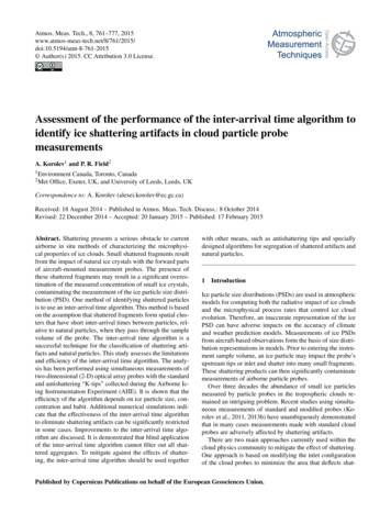
A. Korolev and P. R. Field: Assessment of the performance of the inter-arrival time algorithmFigure 3. Examples of diffraction fringes around out-of-focus images measured by CIP at 15 µm pixel resolution. The diffractionfringes and the particle generating the fringes may be confused withshattered fragments and be rejected by the inter-arrival time algorithm.3.4Figure 4. Examples of out-of-focus images measured by 2-D-S at10 µm pixel resolution. (a) Complete circle out-of-focus images; (b)fragmented out-of-focus images, which were registered in two orthree image frames and identified as shattering artifacts by the interarrival time algorithm. The fragmented out-of-focus images are related to the particles passing through the sample volume near theedge of the depth-of-field.Partially viewed ice branchesMany ice particles develop branches extending from a fewhundred micrometers up to 2–3 mm away from its center(i.e., bullet rosettes, dendrites and aggregated ice particles).The partially viewed branches of such particles could be confused with separate particles possessing short inter-arrivaltime (Fig. 2e), and be identified as artifacts. Rejecting images that are in contact with the edge of the array is one wayto mitigate against this problem.3.5765Diffraction fringesMost particle imaging probes use coherent sources of lightthat result in the formation of diffraction fringes aroundthe image of a particle. The binary representations of thesefringes may manifest themselves as sparse disconnectedpixel images that surround the main particle image. Suchoptical and imaging instrumentation effects may be confused with shattered fragments and result in identifying bothdiffraction fringes and the intact particle producing thesefringes as artifacts.For spherical particles such fringes become most pronounced when the dimensionless distance of the particlesfrom the focal plane is close to Zd 1.9 (Korolev, 2007;his Fig. 9) where Zd 4λZ; λ is the wavelength; Z is theD2distance from the object plane; D is the particle diameter. Non-circular images produce diffraction fringes over awider range of Zd . The probability of imaging the diffractionfringes increases with the increasing pixel resolution. Thus,for probes with coarse pixel resolution 100–200 µm (e.g.,HVPS, PIP, OAP-2DP), diffraction artifacts are quite rare,whereas for probes with 10–15 µm pixel resolution (e.g., 2D-S, CIP) the effect of the diffraction fringes may have a significant effect on misidentification of intact particles as shattering artifacts. A few examples of diffraction fringes aroundthe CIP out-of-focus images are shown in Fig. 3. These images were identified by the inter-arrival time algorithms asshattering artifacts and rejected. The 2-D data are can be tuned to return large images to the pool ofaccepted images. However, setting the threshold for the sizesof the accepted images is ambiguous, and it may result inaccepting shattering artifacts and rejecting intact particles.3.6Out-of-focus fragmented imagesOut-of-focus images of particles traversing the sample areanear the edges of the depth-of-field, when Zd 6 may appearas disconnected images (Korolev, 2007; Fig. 7). If the outof-focus fragmented image has a gap along the flight direction, it may be confused with a shattering artifact. Examplesof the out-of-focus images, which were identified by ITA asshattered fragments, are shown in Fig. 4b. Out-of-focus images, such as images of transparent plates, quite often appearas fragmented and may also be identified by the ITA as artifacts.4Results of measurements of inter-particle distancesBecause shattering generates particles by a very differentphysical process to those that occur naturally, the mode thatdescribes the inter-arrival time distribution of these particlescan be very different to that associated with the natural intact particles, which usually is well described by the Poissondistribution. This difference in the distribution of the particles manifests itself through differing inter-arrival time populations. Therefore, the distribution φ(1t) can be used asone of the metrics for identifying shattering. The purpose ofthis section is to demonstrate the variety of φ(1t) distributions and show their link to the particle size distributions.This consideration is expected to help further understandingof limitations of the ITA.In order to reduce the effect of the air speed u on 1t, theinter-particle distance 1x 1t/u will be used instead of 1t.Accordingly, the distribution φ(1x) and the cut-off-distanceAtmos. Meas. Tech., 8, 761–777, 2015

766A. Korolev and P. R. Field: Assessment of the performance of the inter-arrival time algorithmFigure 5. Comparison of inter-particle distances measured by standard (a) and modified (b) 2DC. Red lines in (a) and (b) indicate the cut-offdistance χ . The distribution of the inter-particle distances for standard (c) and modified (d) probes. Examples of images obtained with anOAP-2DC at 25 µm pixel resolution (e) and an OAP-2DP at 200 µm pixel resolution (f). The measurements were conducted on 1 April duringan ascent through ice cloud from approximately 4600 to 5300 m in the Ottawa region. The temperature varied from 12 to 17 C.χ τ /u will be used instead of φ(1t) and τ , respectively. We will also keep using the conventional term “interarrival time algorithm”, although the term “inter-particle distance algorithm” would be more accurate.4.1Description of the data setThe data used here were collected during the Airborne IcingInstrumentation Evaluation Experiment (AIIE) flight campaign (Korolev et al., 2011, 2013b). The analysis of theinter-particle distance is focused on the measurements oftwo OAP-2DCs installed side-by-side in the NRC Convair580 aircraft. Both instruments have the same pixel resolution 25 µm, optics and electronics. However, one of theprobes had the standard configuration, whereas the secondone had modified arms with the K-tips installed (Korolevet al., 2013a). While K-tips still shatter ice particles, it hasbeen demonstrated that they significantly mitigate the effectof shattering on ice particle measurements. Comparing measurements made with the standard and modified OAP-2DCsbefore and after applying the ITA provides an opportunity toassess the efficiency of the algorithm to successfully identifyand filter out shattering artifacts. The 2-D data were averAtmos. Meas. Tech., 8, 761–777, 2015aged over 5-second time intervals. For most clouds sampledduring the AIIE project such averaging provided statisticallysignificant particle numbers to estimate the function φ(1x)and cut-off-distance χ . In the frame of this study the number of bins in φ(1x) was selected to be 25. This yields areasonable compromise between the statistical significanceof number of counts in each bin and the accuracy of findingχ . Usually, for a typical shape of φ(1x), a number of particle counts over 100 yielded an acceptable estimate of χ for the purposes of this work. A higher number of bins forφ(1x) will require a higher number of counts, and thereforea longer averaging time.4.2Examples of the inter-particle distance distributionThe following three examples are based on the data collectedduring three different flights (1, 8 April 2009) and demonstrate how the presence of large particles and their concentration affect the inter-particle distance distribution φ(1x).The first example demonstrates a moderate level of shatteringand a high concentration of ice. The second example demonstrates more intense shattering and a low concentration of ice.www.atmos-meas-tech.net/8/761/2015/

A. Korolev and P. R. Field: Assessment of the performance of the inter-arrival time algorithm767Figure 6. Examples of the results of the image rejection/acceptance processing with the inter-arrival time algorithm. The images of iceparticles were simultaneously sampled by the standard (left) and modified (right) OAP-2DC during the time period shown in Fig. 5. Greenbackgrounds highlight the images identified by the inter-arrival time algorithm as artifacts. Images with a white background were acceptedby the algorithm. As seen in (a), in some cases the standard OAP-2DC rejects large particles which appear to be intact (red arrows), at thesame time it accepts particles which have the features of shattered fragments (blue arrows).The last example demonstrates a case where shattering has anegligible effect.4.2.1Overlapping modesFigure 5a and c show the time series of inter-particle distances measured by the standard and modified OAP-2DC inan ice cloud. Each inter-particle distance in Fig. 5a and bis represented by a dot. The red lines indicate the cut-offdistances. As seen from these two diagrams, the density ofpoints below the red line is greater for the standard probe(Fig. 5a) than that for the modified one (Fig. 5b). The concentration measured by the modified 2DC, and corrected withthe help of the ITA, varied from 20 to 80 L 1 . Whereas,the uncorrected concentration measured by the standard 2DCvaried from 300 to 1600 L 1 . After applying corrections tothe standard 2DC measurements its concentration varied inthe range 150 to 700 L 1 . The ice particle images measuredby 2DC and 2DP are presented in Fig. 5e and f. Analysis ofthese images shows that the ensemble of ice particles wascomposed of two distinct habits: large spatial dendrites withsizes up to few millimeters and transparent plates with a characteristic size of a few hundred micrometers. The maximumparticle size Dmax calculated for each averaging time intervalremained approximately constant and did not exceed 5 mm.The distributions of the inter-particle distances φ(1x) calculated from the standard and modified 2DC probe data areshown in Fig. 5c and d. The inter-particle distance distribution, φ(1x), for the standard 2DC displays a significant overlap between the long and short inter-arrival modes (Fig. 5c).www.atmos-meas-tech.net/8/761/2015/This may result in rejecting intact particles along with shattered artifacts when 1x χ , and, vice versa, accepting shattered fragments with intact particles for 1x χ .The inter-particle distance distribution φ(1x) for the modified probe has a relatively small overlap between the longand short distance modes, which suggests a better separationof shattered and intact particles. The number of particles associated with the short distance mode for the modified probe(Fig. 5d) is also reduced when compared to Fig. 5b. However, despite the larger separation between the short and longdistance modes, the ITA still identifies large particles, whichappear intact, as shattered fragments (e.g.,

The inter-arrival time distribution in ice clouds was found to have a bimodal shape with modes at 102 and 104 s corre-sponding to approximately 1m and 1cm spatial separations. The particles from the long and short inter-arrival time modes corresponded to estimated concentrations of 0.1-1cm3 and 100cm3 respectively. No conclusions were drawn .