Transcription
Health Sciences M.Sc. ProgrammeApplied BiostatisticsMean and Standard DeviationThe meanThe median is not the only measure of central value for a distribution. Another is thearithmetic mean or average, usually referred to simply as the mean. This is foundby taking the sum of the observations and dividing by their number. The mean isoften denoted by a little bar over the symbol for the variable, e.g. x .The sample mean has much nicer mathematical properties than the median and is thusmore useful for the comparison methods described later. The median is a very usefuldescriptive statistic, but not much used for other purposes.Median, mean and skewnessThe sum of the 57 FEV1s is 231.51 and hence the mean is 231.51/57 4.06. This isvery close to the median, 4.1, so the median is within 1% of the mean. This is not sofor the triglyceride data. The median triglyceride is 0.46 but the mean is 0.51, whichis higher. The median is 10% away from the mean. If the distribution is symmetricalthe sample mean and median will be about the same, but in a skew distribution theywill not. If the distribution is skew to the right, as for serum triglyceride, the meanwill be greater, if it is skew to the left the median will be greater. This is because thevalues in the tails affect the mean but not the median.Figure 1 shows the positions of the mean and median on the histogram of triglyceride.We can see that increasing the skewness by making the observation above 1.5 muchbigger would have the effect of increasing the mean, but would not affect the median.Hence as we make the distribution more and more skew, we can make the mean aslarge as we like without changing the median. This is the property which tends tomake the mean bigger than the median in positively skew distributions, less than themedian in negatively skew distributions, and equal to the median in symmetricaldistributions.VarianceThe mean and median are measures of the central tendency or position of the middleof the distribution. We shall also need a measure of the spread, dispersion orvariability of the distribution.The most commonly used measures of dispersion are the variance and standarddeviation, which I will define below. We start by calculating the difference betweeneach observation and the sample mean, called the deviations from the mean. Someof these will be positive, some negative.1
Figure 1. Histogram of serum triglyceride in cord blood, showing the positionsof the mean and MeanIf the data are widely scattered, many of the observations will be far from the meanand so many deviations will be large. If the data are narrowly scattered, very fewobservations will be far from the mean and so few deviations will be large. We needsome kind of average deviation to measure the scatter. If we add all the deviationstogether, we get zero, so there is no point in taking an average deviation. Instead wesquare the deviations and then add them. This removes the effect of plus or minussign; we are only measuring the size of the deviation, not the direction. This gives usthe sum of squares about the mean, usually abbreviated to sum of squares. In theFEV1 example the sum of squares is equal to 25.253371.Clearly, the sum of squares will depend on the number of observations as well as thescatter. We want to find some kind of average squared deviation. This leads to adifficulty. Although we want an average squared deviation, we divide the sum ofsquares by the number of observations minus one, not the number of observations.This is not the obvious thing to do and puzzles many students of statistical methods.The reason is that we are interested in estimating the scatter of the population, ratherthan the sample, and the sum of squares about the sample mean is not proportional tothe number of observations. This is because the mean which we subtract is alsocalculated from the same observations. If we have only one observation, the sum ofsquares must be zero. The sum of squares cannot be proportional to the number ofobservations. Dividing by the number of observations would lead to small samplesproducing lower estimates of variability than large samples from the same population.In fact, the sum of squares about the sample mean is proportional to the number ofobservations minus one. If we divide the sum of squares by the number ofobservations minus one, the measure of variability will not be related to the samplesize.The estimate of variability found in this way is called the variance. The quantity iscalled the degrees of freedom of the variance estimate, often abbreviated to df or DF.We shall come across this term several times. It derived from probability theory andwe shall accept it as just a name. We often denote the variance calculated from asample by s2.2
For the FEV data, s2 25.253371/(57 – 1) 0.449. Variance is based on the squaresof the observations. FEV1 is measured in litres, so the squared deviations aremeasured in square litres, whatever they are. We have for FEV1: variance 0.449litres2. Similarly, gestational age is measured in weeks and so the gestational age:variance 5.24 weeks2. A square week is another quantity hard to visualise.Variance is based on the squares of the observations and so is in squared units. Thismakes it difficult to interpret. For this reason we often use the standard deviationinstead, described below.Standard deviationThe variance is calculated from the squares of the observations. This means that it isnot in the same units as the observations, which limits its use as a descriptive statistic.The obvious answer to this is to take the square root, which will then have the sameunits as the observations and the mean. The square root of the variance is called thestandard deviation, usually denoted by s. It is often abbreviated to SD.For the FEV data, the standard deviation 0.449 0.67 litres. Figure 2 shows therelationship between mean, standard deviation and frequency distribution for FEV1.Because standard deviation is a measure of variability about the mean, this is shownas the mean plus or minus one or two standard deviations. We see that the majority ofobservations are within one standard deviation of the mean, and nearly all within twostandard deviations of the mean. There is a small part of the histogram outside themean plus or minus two standard deviations interval, on either side of thissymmetrical histogram.For the serum triglyceride data, s 0.04802 0.22 mmol/litre. Figure 3 shows theposition of the mean and standard deviation for the highly skew triglyceride data.Again, we see that the majority of observations are within one standard deviation ofthe mean, and nearly all within two standard deviations of the mean. Again, there is asmall part of the histogram outside the mean plus or minus two standard deviationsinterval. In this case, the outlying observations are all in one tail of the distribution,however.For the gestational age data, s 5.242 2.29 weeks. Figure 4 shows the positionof the mean and standard deviation for this negatively skew distribution. Again, wesee that the majority of observations are within one standard deviation of the mean,and nearly all within two standard deviations of the mean. Again, there is a small partof the histogram outside the mean plus or minus two standard deviations interval. Inthis case, the outlying observations are almost all in the lower tail of the distribution.In general, we expect roughly 2/3 of observations or more to lie within one standarddeviation of the mean and about 95% to lie within two standard deviations of themean.3
Figure 2. Histogram of FEV1 with mean and standard deviation marked.Frequency2015105023x-2sx-s4x56x 2sx s FEV1 (litre)Figure 3. Histogram of serum triglyceride with positions of mean and standarddeviation markedFrequency8060402000.511.52x-2sxx 2s Triglyceridex-sx sFrequencyFigure 4. Histogram of gestational age with mean and standard deviationmarked.5004003002001000x-s x sx-2s x x 2s202530354045Gestational age (weeks)4
Figure 5. Distribution of height in a sample of pregnant women, with thecorresponding Normal distribution curveFrequency3002001000140150160170Height (cm)180190Spotting skewnessHistograms are fairly unusual in published papers. Often only summary statisticssuch as mean and standard deviation or median and range are given. We can usethese summary statistics to tell us something about the shape of the distribution.If the mean is less than two standard deviations, then any observation less than twostandard deviations below the mean will be negative. For any variable which cannotbe negative, this tells us that the distribution must be positively skew.If the mean or the median is near to one end of the range or interquartile range, thistells us that the distribution must be skew. If the mean or median is near the lowerlimit it will be positively skew, if near the upper limit it will be negatively skew.For example, for the triglyceride data, median 0.46, mean 0.51, SD 0.22, range 0.15 to 1.66, and IQR 0.35 to 0.60 mmol/l. The median is less than the mean andthe mean and median are both nearer the low end of the range than to the high end.These are both indications of positive skewness.These rules of thumb only work one way, e.g. the mean may exceed two standarddeviations and the distribution may still be skew, as in the triglyceride case. For thegestational age data, the median 39, mean 38.95, SD 2.29, range 21 to 44,and IQR 38 to 40 weeks. Here median and mead are almost identical, the mean ismuch bigger than the standard deviation, and median and mean are both in the centreof the interquartile range. Only the range gives away the skewness of the data,showing that median and mean are close to the upper limit of the range.The Normal DistributionMany statistical methods are only valid if we can assume that our data follow adistribution of a particular type, the Normal distribution. This is a continuous,symmetrical, unimodal distribution described by a mathematical equation. I shallomit the mathematical detail. Figure 5 shows the distribution of height in a largesample of pregnant women. The distribution is unimodal and symmetrical. TheNormal distribution curve corresponding to the height distribution fits very wellindeed. Figure 6 shows the distribution of FEV1 in male medical students. TheNormal distribution curve also fits these data well.5
05Frequency101520Figure 6. Distribution of FEV1 in a sample of male medical students, with thecorresponding Normal distribution curve234FEV1 (litres)56For the height data in Figure 5 the mean 162.4 cm, variance 39.5 cm2, and SD 2.3 cm. For the FEV data in Figure 6, mean 4.06 litres, variance 0.45 litres2, andSD 0.67 litres. Yet both follow a Normal distribution. This can be true because theNormal distribution is not just one distribution, but a family of distributions. Thereare infinitely many members of the Normal distribution family. The particularmember of the family that we have is defined by two numbers, called parameters.Parameter is a mathematical term meaning a number which defines a member of aclass of things. The parameters of a Normal distribution happen to be equal to themean and variance of the distribution. These two numbers tell us which member ofthe Normal family we have. So to draw the Normal distribution curve which bestmatches the height distribution, we find the mean and variance of height and then usethese are parameters to define which member of the Normal distribution family weshould draw on the graph. We shall meet several such distribution families in thismodule.The particular member of the Normal family for which mean 0 and variance 1 iscalled the Standard Normal distribution. If we subtract the mean from a variablewhich has a Normal distribution, then divide by the standard deviation (square root ofthe variance) we will get the Standard Normal distribution.The Normal distribution, also known as the Gaussian distribution, may be regardedas the fundamental probability distribution of statistics. The word ‘normal’ here is notused in its common meaning of ‘ordinary or common’, or its medical meaning of ‘notdiseased’. The usage relates to its older meaning of ‘conforming to a rule or pattern’.It would be wrong to infer that most variables are Normally distributed, though manyare.The Normal distribution is important for two reasons.1. Many natural variables follow it quite closely, certainly sufficiently closely forus to use statistical methods which require this. Such methods include t tests,correlation, and regression.2. Even when we have a variable which does not follow a Normal distribution, ifwe the take the mean of a sample of observations, such means will follow aNormal distribution.6
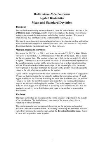
Figure 7. Simulation study showing the effect of taking the average of severalvariablesSingle Uniform 002000-.2 0 .2 .4 .6 .8 1 1.2Uniform variable-.2 0 .2 .4 .6 .8 1 1.2Mean of twoFour Uniform variablesTen Uniform variables15002000150010005000FrequencyFrequencyTwo Uniform variables10005000-.2 0 .2 .4 .6 .8 1 1.2Mean of four-.2 0 .2 .4 .6 .8 1 1.2Mean of tenThe second comment deserves a bit more explanation. To be more precise, if we haveany series of independent variables which come from the same distribution, then theirsum tends to be closer and closer to a Normal Distribution as the number of variablesincreases. This is known as the central limit theorem. As most sets ofmeasurements are observations of such a series of random variables, this is a veryimportant property. From it, we can deduce that the sum or mean of any large seriesof independent observations follows a Normal Distribution.Such a claim deserves some evidence to back it up. For example, consider theUniform or Rectangular Distribution. This is the distribution where all valuesbetween two limits, say 0 and 1, are equally likely and no other values are possible.Figure 7 shows the histogram for the frequency distribution of 10000 observationsfrom the Uniform Distribution between 0 and 1. It is quite different from the NormalDistribution with the same mean and variance, which is also shown. Now suppose wecreate a new variable by taking two Uniform variables and finding their average. Theshape of the distribution of the mean of two variables is quite different to the shape ofthe Uniform Distribution. The mean is unlikely to be close to either extreme, andobservations are concentrated in the middle near the expected value. The reason forthis is that to obtain a low mean, both the Uniform variables forming it must be low;to make a high mean both must be high. But we get a mean near the middle if thefirst is high and the second low, or the first is low and second high, or both first andsecond are moderate. The distribution of the mean of two is much closer to theNormal than is the Uniform Distribution itself. However, the abrupt cut-off at 0 andat 1 is unlike the corresponding Normal Distribution. Figure 7 also shows the resultof averaging four Uniform variables and ten Uniform variables. The similarity to theNormal Distribution increases as the number averaged increases and for the mean often the correspondence is so close that the distributions could not easily be told apart.7
Relative frequencydensityFigure 8. Three members of the Normal distribution family, specified by theirparameters, mean and variance.4.3.2.10-5-4-3-2-1 0 1 2 3 4 5 6 7 8 9 10Normal variableMn 0, Var 1Mn 3, Var 4Mn 3, Var 1Relative frequencydensityFigure 9. Three members of the Normal distribution family with by their meansand standard deviations.4.3.2.10-5-4-3-2-1 0 1 2 3 4 5 6 7 8 9 10Normal variableMn 0, SD 1Mn 3, SD 2Mn 3, SD 1We are often able to assume that averages and some of the other things we calculatefrom samples will follow Normal distributions, whatever the distribution of theobservations themselves.Figure 8 shows three members of the Normal distribution family, the StandardNormal distribution with mean 0 and variance 1 and those with mean 3 andvariance 1 and with mean 3 and variance 4. We can see that if we keep thestandard deviation the same and change the mean, this just moves the curve along thehorizontal axis, leaving the shape unchanged. If we keep the mean constant andincrease the standard deviation, we stretch out the curve on either side of the mean.As variance is a squared measure, it is actually easier to talk about these distributionsin terms of their standard deviations, so Figure 9 shows the same distributions withtheir standard deviations. If we look at the curve for mean 0 and SD 1, we cansee that almost all the curve is between –3 and 3. (In fact, 99.7% of the area beneaththe curve is between these limits.) If we look at the curve for mean 3 and SD 1,we can see that almost all the curve is between 0 and 6. This is within 3 on either8
side of the mean (which is also 3). If we look at the curve for mean 3 and SD 2,we can see that almost all the curve is between –3 and 9. This is within 6 on eitherside of the mean, which is equal to 3 standard deviations. In terms of standarddeviations from the mean, the Normal distribution curve is always the same.To get numbers from the Normal distribution, we need to find the area under thecurve between two values of the variable, or equivalently below any given value ofthe variable. This area will give us the proportion of observations below that value.Unfortunately, there is no simple formula linking the variable and the area under thecurve. Hence we cannot find a formula to calculate the relative frequency betweentwo chosen values of the variable, nor the value which would be exceeded for a givenproportion of observations.Numerical methods for calculating these things with acceptable accuracy have beenfound. These were used to produce extensive tables of the Normal distribution. Now,these numerical methods for calculating Normal frequencies have been built intostatistical computer programs and computers can estimate them whenever they areneeded. Two numbers from tables of the Normal distribution:1. we expect 68% of observations to lie within one standard deviation from themean,2. we expect 95% of observations to lie within 1.96 standard deviations from themean.This is true for all Normal distributions, whatever the mean, variance, and standarddeviation.Martin Bland10 August 20069
standard deviations of the mean. There is a small part of the histogram outside the mean plus or minus two standard deviations interval, on either side of this symmetrical histogram. For the serum triglyceride data, s 0.04802 0.22 mmol/litre. Figure 3 shows the position of the mean and standard deviation for the highly skew triglyceride data.