Transcription
1The Potts ModelA.D. Rollett9th Feb. 2012Based on a lecture for : NATO Workshop on Thermodynamics,Microstructures and Plasticity,September, 2002CarnegieMellonMRSECDiscussions with: K. Okuda, M. Upmanyu, E.A. Holm,M. Miodownik, D.J. Srolovitz, B. Radhakrishnan, G.Rohrer, D. Saylor
References!1.2.3.4.5.A.D. Rollett and P. Manohar, “Continuum ScaleSimulation of Engineering Materials: Fundamentals–Microstructures-Process Applications ” Edited byD. Raabe, F. Roters, F. Barlat, L.Q. Chen, WileyVCH Verlag, Chapter 4 (2004). "http://en.wikipedia.org/wiki/Poisson e Markov process"G.N. Hassold and Elizabeth A. Holm, Computers inphysics, Vol. 7, No.1, Jan/Feb (1993)."Abhijit P. Brahme, Chris Roberts, Shengyu WangPhD theses, Carnegie Mellon University."2
Monte Carlo Method!Square 3D grid8197202229211015163561817423121126Number of nearestneighborsTotal number ofspins/grains241141325Grain Boundary EnergyStored Energy1-6 : six 1st nearest neighbors7-18 : twelve 2nd nearest neighbors19-26 : eight 3rd nearest neighborsGrain BoundaryMobility3
4Potts model!113 113 113 113 113 210 210 210 210 210113 113 113 113 113 210 210 210 210 210113 113 113 113 113 210 210 210 210 210113 113 113 113210 210 210 210 210113 113 113 113 210 210 210 210 210 210113 113 113 113 210 210 210 210 210 210113 113 113 210 210 210 210 210 210 2102 unlike nearest neighbors6 unlike next nearest neighborsN n(E J(Si , S j ) 1 δ Si S jj i)E system energyP transition probabilityJ interaction energyµ mobilityS orientationJ(Si ,S j ) µ (Si , S j ) 1 Jµ max.P J (S , S ) max. ΔE ij µ (Si ,S j ) exp T µ max. Jmax.ΔE 0ΔE 0
5Modification for variable lattice T! Large ( 2) variation in grain boundary energy withfinite lattice temperature can lead to excessiveroughness of a low energy boundary." Variable lattice temperature used to ensure uniformroughness on all boundaries because a large rangein g.b. energy required (Read-Shockley, e.g.)." Abnormal grain growth investigations have alsosuggested scaling the lattice temperature based onthe local grain boundary energy (all in 2D)." This has been found to allow the model to correctlymatch the expected variation in shrinkage rates ofisolated (circular) grains, and to match the predictedabnormal growth of polycrystalline structures(Radhakrishnan)."
6MC method: temperature scaling! J ( Si ,S j ) M (Si , Sj ) J maxMmaxConventional:P(Si ,S j ,ΔE, T ) J S ,S M S ,S( i j ) ( i j ) exp( ΔE kT ) Mmax J max J (Si , Sj ) M (Si ,S j )Temperature JmaxM maxScaling:P(Si ,S j ,ΔE, T ) ΔE J (Si ,S j ) M( Si ,S j ) exp JMmax kTJ (Si ,S j ) maxΔE 0ΔE 0ΔE 0ΔE 0
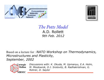
7Test: columnar growth!Migration"direction"Fixed TemperatureTemperature γ
8Temperature scaling: shrinking circle results!Lattice: square, with 1st and 2nd nearest neighbors (wild flips allowed)Ratio of Shrinkage Rates1M, standard T 0E, standard T 0E, standard T 0.4E, modified T 0.4M, modified T 0.40.80.60.40.200Data.circles 11 ix 010.20.40.6Mobility, or Energy ratio0.81
Parallel Monte Carlo AlgorithmThe algorithm is a modification of the original Ising model. System Energy (E): Spin-flip probability (p): Single Processor sweep sequence:1. Pick a site at random2. Pick a new spin value from one of its neighbors3. Calculate ΔE4. Accept or reject change based on p(ΔE)
Parallel Monte Carlo Algorithm Division of microstructure into subdomainsBoundary Sites? Use GHOST CELLSIllegal Flips? Apply checkerboard masksSynchronous? Update processors at common points Multi-processor Sweep Sequence:Start Color Loop(B, HS, DS, W) Loop over lattice sites of color I1.a. Pick a site at randomb. Pick new spin valuec. Calculate ΔEd. Accept or reject change 2. Exchange boundary information with neighbor processors End lattice site loop End Color LoopW. Gropp et al., Using MPI-2, 1999. S.A. Wright et al., Sandia Report#SAND97-1925.
Inter-processor CommunicationHow do processors send information? 1. Call to MPI library function returns information about 6 neighbors (North, South, East, West, Up, Down)2. Information can be sent to neighbor by specifying destination as (nodenorth,nodesouth, nodeeast, nodewest, nodeup, nodedown)UpNorthAWestSouthDownEast
Inter-processor Communication01AB01xx 1Processor A sends its boundary sites to the right (processor B).Information stored in “ghost cells” of B[I 0,j]Reversal: B sends its boundary sites to the left (processor A).Information is stored in “ghost cells of A[imax 1,j]
Model ValidationObjective: To determine whether this PMC algorithm can reproduce curvaturedriven grain growth.3000Linear relationshipexists between area andtime.Area25002000150010005000050100150200Time (MCS)250300350
Model ValidationPARAMETERS: 2003 box T 1.7 Initial Radius 50 Isotropic Grain Boundary PropertiesResults confirm the sphere is shrinking inan isotropic manner towards its center ofcurvature.Parallel MC algorithm obeysconditions for curvature-drivengrain growth; PMC will be usedto simulate grain growth.
Efficiency and ScalabilityObjective: To determine the scalability and efficiency of a synchronousparallel Monte Carlo algorithm as a function of the number of processorsand processor workload on a supercomputing and beowulf network.Nomenclature:msca01Machine:m mrsecl lemieuxr robertsVariables:1. # Processors 2. Workload 3. HardwareStyle:eff efficiencysca scalabilityRun #:
ScalabilityMaintain a constant subdomain size as more processors are added.Total timeMSSSmemorySubtracted I/O timeIn theory, a perfectly scalableprocessesprogram will be able to finish asimulation run in the same timefilegiven each processorhas the sameworkload.I/O Operation:However, portions of the algorithmEachslave innodesendsarrayare serialnature(i.e.must beinformationmaster node.completed tosequentially).Master node writes to file.
Efficiency Maintain a constant TOTAL domain while increasing the number of processors.Q:InIftheory,a man acandig relationshipa hole in 60linearminutes,can 60men diga hole inshould existbetweenspeed-up1 timeminute?and the number ofprocessors.Physical limitations exist which remove thiscurve from a linear relationship. Mostcommon culprit is “interprocessorcommunication”!!For our experiment, a near-linear relationship exists upto 256 processors.
Memory Performance Cache Performance Cache Definition: A memory area where frequently accessed data can bestored for rapid access1.7% Miss rate determined for PMC codePSC Standard lists 10% as poor Cache usage MFLOPs Performance MFLOPs Definition: MFLOPS is an abbreviation of floating pointoperations per second. This is used as a measure of a computer'sperformance, especially in fields of scientific calculations that make heavyuse of floating point calculations.
Grain Growth StudyObjective: Determine kinetic behavior for isotropic and anisotropic grainboundary properties.1. Self Similarity – structure looks identical to previous state if examined at adifferent magnification.2. Grain Growth KineticsTheoretical calculations yield n 1. Values close to 1 have beenfound for very pure metals annealed close to their melting points.3. Unimodal Grain Size DistributionsS.L. Semiatin J.C. Soper, I.M. Sukonnik, Acta Mater., Vol. 44, No. 5, p. 1979
Grain Growth Study Evolution of microstructure using isotropic GB propertiest 10 MCSt 500 MCSt 1000 MCS
21Texture Description! Monte Carlo Model works with a set of discrete orientations Conventional: scalar parameter, S (1.Q), spin number Texture: assign (3-parameter) orientation, gi(Ψ,Θ,φ) toeach spin number, Si: Ψ,φ (0.2π), Θ (0.π/2) Calculate the disorientation for each combination of grains and associatedproperties. Make a look-up table of all required properties before starting evolutionsimulation.S1S2(Ψ1,Θ1,φ1) (Ψ2,Θ2,φ2)S1S2::Sn-.Sn(Ψn,Θn,φn) g12 g1n- g2n-
Simulation: kinetic Monte Carlo! Triangular 200 x 200 grid, 1st & 2nd nearestneighbors, Q 500, spin no. linked to orientation." Equiaxed initial grain structure with 4000 grains." G.B. properties forS1S2.Snunalloyed Al,(Ψ , Θ , φ ) (Ψ , Θ , φ )(Ψ , Θ , φ )γ( g12),γ( g1n),S1as measured."11Energy, Mobility222-::Sn0.8EnergyMobility0.61M( g12)S2c1 c0/15.*(1.-ln(c0/15.))1nnnM( g1n)γ( g2n),M( g2n)-0.40.20c2 1.-0.99*exp(-.5*(c0/15) 9)051015Angle ( )2025(M M0 1 0.99e 0. 5(θ θ 0 )9)22
Grain Growth StudyExponent value indicatesmicrostructure is coarsening too fast.Source of problem?MC is a stochastic model, whichimplies random events must occur.By selecting the checkerboardrandomly, the exponent has beenreduced by 0.25!!!
Grain Growth Study UPDATE Evolution of microstructure using isotropic GB properties Closer agreement with the ideal case. The change in area should be linearlyproportional to time (n 1.0)400300n 1.0820010000200400600Time (MCS)800
Model Validation2003 box T 1.5 Isotropic Grain Boundary Properties50 MCS70 MCS100 MCS200 MCSResults confirm the sphere is shrinking in an isotropic manner Temperature parameter should be equal to or greater than 1.5
Model ValidationObjective: To determine whether this PMC algorithm can reproduce curvaturedriven grain growth.2v MγR9000spherD (T 1.5)spherG (T 1.5, p(dE 0) 0.5)spherH (T 0.0, p(dE 0) 0.5)Linear relationshipexists between area andtime.Sphere Area 0400Time (MCS)500600700800
Grain Growth Study Grain Size Distribution is invariant with time0.140.1210 MCS20 MCS30 MCS0.140 MCS50 MCSFrequency60 MCS70 MCS0.0880 MCS90 MCS100 MCS200 MCS0.06300 MCS400 MCS500 MCS600 MCS0.04700 MCS800 MCS900 MCS1000 MCS0.02000.511.522.5R/ R Peak fluctuations occur at late times when NG is small.
N-fold way model! Concepts"-Poisson Processes "-Continuous time" Monte Carlo Simulation Algorithms"– Metropolis (conventional)"– N-fold Way" Connection between Poisson Processand “N-fold way” model" Summary"28
Poisson Processes! A Poisson process is a stochastic process which is defined in termsof the occurrences of events. Also, the number of events betweentime a and time b is given as N(b) N(a) and has aPoisson distribution."The probability that there are exactly k occurrences during unit time(k being a non-negative integer, k 0, 1, 2, .) is"Where"e is the base of the natural logarithm (e 2.71828.) "k is the number of occurrences of an event "k! is the factorial of k "λ is a positive real number, equal to the expected number ofoccurrences that occur during the given interval."Note: This probability distribution may be deduced to!29
Examples of Poisson Processes! The number of telephone calls arriving at aswitchboard per hour. " The number of webpage requests on a server, exceptfor denial of service attacks ." The number of photons hitting a photodetector, whenlit by a laser source. " The number of particles emitted via radioactive decayby an unstable substance. " Spin flippings in Monte Carlo n-fold way model ( ourfocus)"30
General characteristics of a Poisson process!There are only two conditions for astochastic process to be a Poisson process."1. Orderliness: "Arrivals donʼt occur simultaneously."2. Memorylessness:"The number of arrivals occurring in any boundedinterval of time t is independent of the number ofa r r i v a l s o c c u r r i n g b e f o r e t i m e t ".31
Continuous time!In probability theory, a continuous-timeMarkov process is a stochastic process { X(t) : t 0 }that satisfies the Markov property and takes values froma set called the state space. "The Markov property states that at any time s t 0, theconditional probability distribution of the process at times given the whole history of the process up to andincluding time t, depends only on the state of the processat time t."32
Monte Carlo Simulation-- Metropolis Algorithm!The key steps of this algorithm are as given below (Landau and Binder2000):"1. Choose a site i at random"2. Calculate the energy change associated with changing the spin at the ithsite"3. Generate a random number r such that 0 r 1"4. If r exp(-ΔE/kBT), flip the spin "5. Increment time regardless of whether a site changes its spin or not"6. Go to 1 until sufficient data is gathered."Disadvantages: During the late stages of evolution the transition probabilityapproaches 0 at most sites. For low temperatures, flipping probability is low.33
Steps of n-fold way algorithm!1.2.Generate a random number r (0,1] ."Choose a class k that satisfies the condition given inEquation "3.Generate a random number to choose one of the sitesfrom class k"Flip the spin at the chosen site with probability 1"Update the class of the chosen spin and all of itsnearest neighbors"Determine activity Qn"4.5.6.7.Go to 1 until sufficient data is gathered"Advantage: Eliminate the need to unsuccessful changes bycalculating the spin-flip transition probability for each of thelattice sites before choosing a site to flip for a given state of the34system.
A specific case of Poisson Process!A Poisson process is characterized by a rate parameterλ, also known as intensity.PλProbability of occurrence vs. time.t35
Derivation of Time increment (Link)!In the n-fold way, every spin flip attempt is successful, so the n-fold way time"increment must be scaled by the average time between successful flips in the"conventional Monte Carlo scheme."Probability that no successful flip has occurred in the time interval Δt"Probability that no successful flip has occurred in the time interval Δt dt"Poissondistribution!36
Summary! Monte Carlo n fold way algorithm canbe effectively treated as a Poissonprocess." Continuous time is applied in MonteCarlo simulation. " Monte Carlo n-fold way algorithm ismore efficient for relatively hightemperatures or in larger data sets thanconventional models. "37
An example of classes (Ising Model)!4 Nearest neighbors (z 4) and J H 1,and KBT 0.4.38
Link “n-fold way” to Poisson Process!In effect, the time increment, Δt, in the n-fold way algorithm iscorrelated to the probability that the given system configurationwill change to a different configuration during the time increment:"This equation is based on the assumption that the successful reorientation of a site is described by an exponential probabilitydistribution."Hence, successive evolution steps are Poisson events.!39
40Simulation Approach! 2D Monte Carlo model for grain growth: 200x200 triangularlattice; Q 500; lattice temperature 0.35, scaled by energyfor constant boundary roughness; 2000 grains coarsen to 200 grains; 3D orientations. 3D Monte Carlo model: 100x100x100 domain with a (1,2,3)neighbor simple cubic lattice, temperature 0.9 (some at 0.5;little sensitivity to lattice temperature); 10,000 grains at t 0. Texture mapped to a list of 500 discrete orientations; fccrolling texture with 6% near-cube grains added. Anisotropic grain boundary properties incorporated to modifythe energy and mobility; values taken from experiment (lowangle boundaries) and simulation (molecular dynamics byUpmanyu, Srolovitz at Princeton). Simulated annealing used to optimize placement of cubegrains.
Grain Size Control! Upper right panel illustrates the physicsof boundary-particle interaction: Dpinned dppt/Vf"Lower right panel shows summary ofexperimental data, together with onlyavailable parallel calculations withMonte Carlo in 3D."Investigating the significant range ofparticle volume fraction drives us intothe petascale; linear sizes of therequired mesh indicated on graph."Monte Carlo method (Potts) offers onlypractical algorithm."CMU parallel results: RobertsPrevious parallel results: RadhakrishnanPrevious parallel results: MiodonwikExperimental review: Manohar et al. 1998
Particle Induced Abnormal Grain GrowthThe objective of the research was to examine the affect of non-randomparticle placement on the kinetics and limiting grain size. During thecourse of the inverstigation, abnormal grain growth (AGG) wasobserved in a few of the microstructures.Microstructures were generated with an equiaxed morphology and anarrow grain size distribution (i.e. Rmax did not exceed 2.5 R ). In asubsequent step, the microstructures were injected with inert, monosized particles. The particles were not randomly inserted, butpreferentially placed on grain boundaries in specific fractions.The simulations were conducted using a parallel version of the Pottsbased Monte Carlo algorithm. Digital microstructures were 4003voxels in volume and isotropic grain boundary properties were applied(γ 1, M 1).
List of configurations examined in the research project.Ex: 0.04VV and 0.03 fraction on grain boundaries.With 0.04VV of cubic particles (volume 27 voxels), themicrostructure contains approximately 95,000 particles. Ofthese 95,000 particles, 30% or 28,500 will be situated on thegrain boundaries and the remaining 70% will be located in thegrain interiors.
Two-dimensional cross-section taken from thecenter of the modeling domain. An example ofNGG and AGG is provided.(Note: Time steps are logarthmic)R0 7.6, 0.04VV, and 70% ofparticles on grain boundariesR0 18.4, 0.06VV, and 30% ofparticles on grain boundaries
In the simulations withNGG, the pinned grainsize is well below theZener threshold; on theother hand, the AGG casedoes not have a limitingsize.The average growth ratedoes not behave in a similarfashion to other simulationsexhibiting only NGG andboundary pinning.Predicted DL (4r/3f)
In the abnormal case, the GSD appears to be uni-modal, but asecondary peak becomes apparent at late times.
SummaryAbnormal grain growth is observed in a particle-containingmicrostructure.Isotropic grain boundary properties eliminate texture as a possiblesource for AGG.AGG appears to be caused by a combination of grain size and localparticle density fluctuations on grain boundaries.
484: Critical dispersion in orientation! Abnormal grain growth is significant in the early stages ofrecrystallization of metals: coarsening of subgrain structurescan generate nucleation. For coarsening within a single orientation (i.e. a subgrainstructure) there appears to be a critical dispersion (spread) intexture.- Narrower dispersions lead to regular (self-similar)coarsening.- Larger dispersions lead to quasi-recrystallization.- At the critical dispersion, abnormal growth occurs. Measured properties used for low angle boundaries in Al, i.e.energy and mobility. Detailed analysis by Miodownik on subgrain structures withsmall mean misorientations: same result. Experiments by Ferry and Humphreys suggest that thisbehavior is observed experimentally.
49Single Component Dispersion(Mosaic Spread)!1.2Frequency1Freq. (4 )Freq. (8 )Freq. (13 )0.80.6FWHM0.40.200dispersion.anal.Kdata 10 vi 0151015Deviation ( )202530
50Sma'dispersion:4 FWHM!1.2Frequency1Freq. (4 )Freq. (8 )Freq. (13 )0.80.6FWHM0.40.200dispersion.anal.Kdata 10 vi 0151015Deviation ( )202530
51Intermediatedispersion :8 FWHM!1.2Frequency1Freq. (4 )Freq. (8 )Freq. (13 )0.80.6FWHM0.40.200dispersion.anal.Kdata 10 vi 0151015Deviation ( )202530
52Broaddispersion :13 FWHM!1.2Frequency1Freq. (4 )Freq. (8 )Freq. (13 )0.80.6FWHM0.40.200dispersion.anal.Kdata 10 vi 0151015Deviation ( )202530
53A max/ A Critical Dispersion!140 Maximum area/ A varies sharply withdispersion. Abnormal grainsacquire largermisorientations.100120Time 5 107 MCS80604020002468101214Standard Deviation ( 810Misorientation121416
54Comparison with theory!2 10-5Rollett & Mullins (1996); Miodownik (2001)dA 2πMγdt1 10-5Γ γabnm/γmatrixµ mabnm/mmatrixρ Rabnm/ Rmatrix d!/dt0-1 10-5SimulationTheoretical 1a(Γ) (6 / π )sin (1/ 2Γ) 3-2 10-5-3 10-5comp02.amax.hist105106time(MCS)dρabnm Mmatrixγ matrix 2 G(ρ, µ, Γ)dt2 Rmatrix ρ 1G( ρ, µ, Γ) µΓ a (a 2) ρ 4
Shrinkage Rates Mobility, or Energy ratio Lattice: square, with 1st and 2nd nearest neighbors (wild flips allowed)! . Call to MPI library function returns information about 6 neighbors ! (North, South, East, West, Up, Down)! 2. Information can be sent to neighbor by specifying destination as (nodenorth, . an isotropic manner towards its .