Transcription
MATLAB Production Server Interface for TIBCO Spotfire SoftwareReference Architecture1
ContentsIntroduction . 3System Requirements . 3MathWorks Products . 3TIBCO Products . 3Reference Diagram . 4Getting Started Guide . 5On the machine that TIBCO Spotfire Server is running: . 5Customizing the Configuration . 5Deploying the MATLAB Production Server Interface for TIBCO Spotfire software . 7Within MATLAB . 11Prototyping Workflow . 12Production Workflow . 14On the TIBCO Spotfire client machines . 15References . 36Contact Information. 36Appendix A: Tool installation . 37Appendix B: Rebuilding the Spotfire Extension . 37Appendix C: Performance Tips . 42TIBCO Spotfire in a clustered configuration. 42MATLAB Production Server in a clustered configuration . 42Appendix D: Modify configuration files . 44Appendix E: MATLAB Function Service Discovery . 45Appendix F: Troubleshooting . 46Appendix G: Code Listings. 47Listing A: MATLAB Demo code for Portfolio Optimization . 47Listing B: Android Application Source . 47Appendix G: Class diagram for MathWorks.MPSExtension . 502
IntroductionSpotfire analytics [1] is a highly visual and open analysis environment that complements packagedapplications. A few clicks combine and visualize multi-sourced information with an array of dynamicallylinked plots that dramatically increase insight and understanding of complex data. Spotfire allows you tocapture reusable analysis methods that clearly and easily lead colleagues through approved steps togather, calculate, visualize and share results.MATLAB [2] is the high-level language and interactive environment used by millions of engineers andscientists worldwide. It lets you explore and visualize ideas and collaborate across disciplines includingsignal and image processing, communications, control systems, and computational finance.MATLAB Production Server [3] lets you run MATLAB programs within your production systems,enabling you to incorporate custom analytics in enterprise applications.This reference architecture details the use of MATLAB as the language of technical computing to expressadvanced analytics and algorithms. The MATLAB algorithms developed in the desktop client can bedeployed in a service-oriented architecture (SOA) to address typical production demands handling thescalability and reliability requirements of business-critical applications.Solutions using such an architecture enables the use of MATLAB’s large and powerful collection ofstatistical and machine learning algorithms and tools for organizing, analyzing and modeling data. Theapplication of this architecture enables a workflow supporting the modeling and visualization of dataand analysis right from prototype to full production usage across large enterprises.System RequirementsThis reference architecture is comprised of the following components and was developed using theversions as listed. See the product documentation for any product specific requirements.MathWorks Products1. MATLAB (R2014b or later)2. MATLAB Compiler (R2014b or later)3. MATLAB Production Server (R2014b or later)TIBCO Products1.2.3.4.TIBCO Spotfire Server (6.0.0 or later)TIBCO Spotfire Web Player (6.0.0 or later)TIBCO Spotfire Professional or Enterprise (6.0.0 or later)(Optional) TIBCO Spotfire Statistical Services3
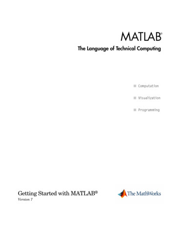
Reference DiagramBelow is a pictorial architecture of the entire system.MathWorks.MPSExtensionCustom component using the SpotfireSDK and the MATLAB ProductionServer .NET Client library enables thetransfer and marshaling of databetween the two systems.The Spotfire environment provides several interfaces [4] to numerous data sources and informationservices. In this architecture, MATLAB is used as a computation service enabling the use of MATLABbased analytics with data from a variety of sources. Results of MATLAB analytics are visualized withSpotfire data visualizations and dashboards on the desktop, mobile or within web browsers.4
Both Spotfire Server1 and MATLAB Production Server2 can be installed in their own standalone orclustered configurations for performance, reliability, fail-over, and disaster recovery. Further discussionon a scaled-out architecture can be found in the Performance Tips in the appendix of this document.Getting Started GuideThis section is designed to enable the user to quickly set up a demo example integrating TIBCO Spotfirewith MATLAB Production Server. Detailed information on Spotfire package deployment, troubleshooting,accessing from mobile applications etc. is available in later sections.On the machine that TIBCO Spotfire Server is running:1. Copy the MathWorks TIBCO Spotfire Extension installer to the machine on which TIBCOSpotfire Server is running and then run the installer. This will create two Spotfire package files inthe folder; 1) MathWorks.MPSExtension.spk and 2) ProtocolBuffers.spkCustomizing the Configuration2. Within the MathWorks.MPSExtension.spk file are two XML files that are used to customize theconfiguration:ServerConfiguration.xml is used to configure the URL address for accessing MATLAB ProductionServerFunctionList.xml defines the list of functions running on MATLAB Production Server.These files contain information visible to the Spotfire client, and must be updated to contain thecorrect information. Reference Appendix D of this document for the process to access the XMLfiles and for rebuild the ‘.spk’ file once the files have been updated.3. Update the ServerConfiguration.xml follow to define the hostname or IP address and port onwhich MATLAB Production Server is listening:1Please see: r.aspxPlease see: -scalability25
The FunctionList.xml file lists the MATLAB functions that can be called from Spotfire. This XML fileshould be modified to include the name of MATLAB function, the input and output parameters, and thedata types. This demo uses the optimisePortfolio MATLAB function. The MATLAB code is listed below,followed by the modified FunctionList.xml file.function weights optimisePortfolio(dates, prices, upperBoundWt)% OPTIMISEPORTFOLIO Simple portfolio optimisation% This demo computes weights of a portfolio defined by a matrix of asset% prices for given dates maximising Sharpe ratio;%% The portfolio weights are bounded by the same scalar value upperBoundWeight% Check inputsdates dates(:);validateattributes(prices, {'numeric'}, {'2d'});validateattributes(upperBoundWt, {'numeric'}, {'scalar'});assert(size(prices, 1) length(dates), .'optimisePortfolio: Size mismatch; Expected number of rows in prices is %d and received is %d', .length(dates), size(prices, 1));% Calculate Returns% Calculate daily returnsassetReturns tick2ret(prices, dates, 'Continuous');%pppp% log returns, Financial TBSetup portfolio Portfolio; p.estimateAssetMoments(assetReturns); %Mean and covariance of asset returns from return data. p.setDefaultConstraints; %Non-negative weights that must sum to 1. p.setBounds(p.LowerBound, upperBoundWt*ones(1, size(prices, 2)));% Find min variance portfolioweights p.estimateMaxSharpeRatio(); FunctionListXMLDocument archive portOpt /archive functionname optimisePortfolio /functionname functionsample System.String[,] weights optimisePortfolio(System.DateTime[] dates,System.Double[,] prices, System.Double upperBoundWeight) /functionsample functionsyntax optimisePortfolio /functionsyntax functionhelp ![CDATA[This function computes weights of a portfolio defined by a matrix of assetprices forgiven dates maximising Sharpe ration; portfolio weights are bounded by the samescalar valueupperBoundWeight. br/ The maximization of the Sharpe ratio is accomplished by a one-dimensionaloptimization usingfminbnd to find the portfolio that minimizes the negative of the Sharpe ratio. Themethodtakes only a fully qualified Portfolio object as its input and uses allinformation in the6object to solve the problem.]] /functionhelp /FunctionListXMLDocument
After modifying the two XML files to reflect the MATLAB functions being deployed, follow directions inAppendix D to recreate the Spotfire package.Deploying the MATLAB Production Server Interface for TIBCO Spotfiresoftware4. To deploy the MATLAB Production Server Interface for TIBCO Spotfire software onto the Spotfiresystem, open the TIBCO Spotfire Server application.7
5. Open the Administration Console.8
6.Select the Deployment Tab.7. Within the “Software Packages” section, use the “Add” button to add the following two fileswhich were extracted from the installer application when it was run:9
MathWorks.MPSExtension.spkProtocolBuffers.spk10
8. Once the two packages are added, select the “Validate” option at the bottom of the page toverify all dependencies. Once you receive the “Validation OK” message, then select “Save”.Within MATLABAs an example of how to use the extension, we shall take a simple portfolio optimization demo problem.Portfolio optimization [5] is the process of choosing the proportions of various assets to be held in aportfolio, in such a way as to the portfolio better than any other per some criterion. The criterion willcombine, directly or indirectly, considerations of the expected value of the portfolio's rate of return aswell as of the return's dispersion and possibly other measures of financial risk.In this demo, MATLAB is used to compute weights of a portfolio defined by a matrix of asset prices forgiven dates maximizing the Sharpe ratio [6]. The portfolio weights are bounded by the same scalar valueas the upper Bound. The Sharpe ratio characterizes performance of an investment asset incompensating the investor for the risk taken. When comparing two assets versus a common benchmark,11
the one with a higher Sharpe ratio provides better return for the same risk (or, equivalently, the samereturn for lower risk).This is a single example of using MATLAB as the computation engine and the choice of example couldjust as easily be rewritten across a number of industries and application areas.Prototyping WorkflowFor the portfolio optimization problem, the function signature looks like:function weights optimisePortfolio(dates, prices, upperBoundWt)9. The first step in building a robust function is to check that our inputs are valid.%% Check inputsdates dates(:);dates cell2mat(dates);prices cell2mat(prices);upperBoundWt cell2mat(upperBoundWt);validateattributes(prices, {'numeric'}, {'2d'});validateattributes(upperBoundWt, {'numeric'}, {'scalar'});assert(size(prices, 1) length(dates), .'optimisePortfolio: Size mismatch; Expected number of rows in pricesis %d and received is %d', .length(dates), size(prices, 1));Leveraging the MathWorks financial toolbox, MATLAB provides a very compact and readable way toexpress many algorithms. This is no exception. Our optimization code looks like:%% Calculate Returns% Calculate daily returnsassetReturns tick2ret(prices, dates, 'Continuous');Financial TB% log returns,%% Setup portfoliop Portfolio;p p.estimateAssetMoments(assetReturns); %Mean and covariance of assetreturns from return data.p p.setDefaultConstraints; %Non-negative weights that must sum to 1.%p p.setBounds(p.LowerBound, upperBoundWt*ones(1, size(prices, 2)));%% Find min variance portfolioweights p.estimateMaxSharpeRatio();Running the code in MATLAB allows users to develop and prototype ideas quickly. Visualization of thedata using the MATLAB desktop based graphics system gives quick and early feedback on algorithmdesigns. For example, to run our function we use asset prices from an XLS spreadsheet. Our data comesfrom historic daily close prices of global large-cap equity indices, from April 1993 to July 2003.12
This dataset contains asset prices from1. . (TSX) Canadian TSX Composite2. (CAC) French CAC 403. (DAX) German DAX4. (NIK) Japanese Nikkei 2255. (FTSE) UK FTSE 1006. (SP) US S&P 500A small sample of this data looks like:Reading in the data and calling the optimization:%% Import Data% Read asset prices from an Excel spreadsheet[prices, , rawData] xlsread('IndexData.xlsx');assetNames rawData(1, 2:end);dates datenum(rawData(2:end, 1), 'dd/mm/yyyy');%% Set parametersupperBoundWeight 0.3;%% Optimise portfolioweights optimisePortfolio(dates, prices, upperBoundWeight);%% Display resultsf ,'S&P'});title('Optimized Asset Allocation');Early and immediate feedback can be visualized in MATLAB.13
This represents a typical prototyping workflow in building data analytics algorithms in MATLAB.When satisfied with the algorithm, the user can democratize the results of the analysis by taking theMATLAB code into production using TIBCO Spotfire.Production WorkflowThe first step in taking the MATLAB function to production is to deploy the code using the MATLABproduction server. This can be done using the deployment tool (deploytool).10. Using the MATLAB Production Server Compiler, specify the function to be packaged andcreate the archive by selecting the “Package” button.14
11. Once complete, copy the resulting ‘.ctf’ file to the auto-deploy folder of MATLAB ProductionServer. Ensure that the MATLAB production Server is running.On the TIBCO Spotfire client machines12. Restart any Spotfire clients and select “Update Now” to update the client with the MATLABProduction Server Interface for TIBCO Spotfire software.15
Installing the update will enable the Spotfire user to access the MATLAB Production Server tool.13.From the Tools menu, select the “MATLAB Production Server” tool.This brings up the tool that will allow configuration of the data function. The inputs include a selectionof available MATLAB Production Server instances as configured earlier allowing users to partition theirenvironment into development, test and production as per best practices.16
The figure above displays the UI for the MATLAB Production Server tool. The first field is the MATLABProduction Server Address. This is the URL of the machine where MATLAB Production server is hostedand is populated using information in the ServerConfiguration.xml file modified in step (3).The second field is the Function Configuration file which contains the list of all MATLAB functionsavailable. This is populated using information in the FunctionList.xml file modified in step (3).Modifying the configuration files after installationOnce the extension is installed, the two XML files(ServerConfiguration and FunctionList) are availablelocally on the end users machine in the path shown under ‘Deployed Function ConfigurationFile’(screenshot below). It is possible for the Spotfire end user to collaborate with the MATLABdeveloper and modify these files individually if changes are required. A second option is for the MATLABdeveloper to make the changes required and repackage the Spotfire updates and push it to all Spotfireend userd17
The ‘Refresh’ button highlighted below allows the Spotfire end user to download the latestFunctionList.XML file directly from the MPS server. To enable this functionality, follow instructions inAppendix E.A prototype definition for the MATLAB function to be called enables marshaling of datatypes anddimensionalities between the two environments. The specification of the prototype uses the followingsyntax:18
In our example, our MATLAB syntax:weights optimisePortfolio(dates, prices, upperBoundWt)would translate to:[System.Double[] weights] optimizePortfolio(System.DateTime[] dates, System.Double[,]prices, System.Double upperBound)This can be roughly read as: “Call the optimisePortfolio function providing a Column (vector) of date/timevalues, a Table (array) of Doubles, and a single scalar Double as an upper bound weight. The function willreturn a Column (vector) of weights as an output”.Pressing the Add to Data Functions button will add the algorithm to the current document’s list of datafunctions.Clicking the OK button closes the GUI. The list of data functions is available in the documents properties.19
14. From the “Edit” menu, select the “Data Function Properties”, and select “Edit Parameters”.Map the data columns from the current document to the function’s parameters as appropriate (Input),and setup the data function to create a new Data Table using the results received from MATLABProduction Server (Output).Each individual input and output can now be mapped, to the appropriate columns and table in thedocument. For example, the dates input is mapped to the Dates column of the IndexData table.20
The prices input comes multiple columns from the IndexData table:21
The upperBound input is mapped to a single scalar Double value 0.3.22
The output is configured to create a new data table.Finally, the entire function is marked to “Refresh automatically”. At this point, we have a fully configuredfunction and any selection of the data will call the MATLAB function and create a new visualization. TheMATLAB portfolio optimization code is now executed on every selected/marked point on thevisualization in TIBCO Spotfire.23
24
15. After “marking” or selecting a section of data, the new Data Table reference will be availablewithin the document for use with any of the Spotfire visualization tools.16. Add new visualizations using the “Output” data25
17. Finish your document and publish it for use by others using the web and mobile clients.26
Web UsersMaking the analysis developed above available on the network via a Browser is now possible using theTIBCO Spotfire Web Player. The Web player uses the same extension code to call MATLAB to provideinteractive dashboards available off a web browser. To make the analysis available via to Web users whowill not need any special client side tooling. To do this, the analysis is saved to the Library making itavailable to all users of the Spotfire Server.The tool will prompt for a filename and a few other minor details such as description. The publicationprocess should be close to a few clicks at most.The Spotfire WebPlayer now provides the analysis on a regular JS enabled internet browser. Shownbelow is MATLAB powered interactive analysis available in a standard Web Browser (Chrome).27
Clicking on the analysis brings up the MATLAB powered dashboard in a Web Browser.28
This technique enables multiple users to concurrently access the analysis. Every click of the interactivevisualization calls our optimization MATLAB code. The scalability of the back-end infrastructure ispossible by using load-balancers both for the TIBCO Spotfire servers as well as the MATLAB ProductionServers as per recommended best-practices for the IT setup of these infrastructure stacks.Mobile Platform UsersThe TIBCO Spotfire stack offers tools such as tibbr [7] for the collaboration aspects of making theresults of data analysis widely available. However, given the availability of the MATLAB powereddashboard as a pure-client side visualization, it is also possible to create custom branded applicationsthat leverage the availability of the analysis as a Web applications that leverage the WebView in iOS [8]and Android [9] powered devices.As an example, we will create a custom Android application that exposes the MATLAB computationthrough an Android device. This example uses the Android Software Development Kit [10].Start a new Android application project from the menu.Provide a name for the application and package to configure the application.29
It is also possible to brand the application with custom look/feel themes but discussion of that is outsidethe scope of this document.30
For this example, we will just use a blank template:31
The analysis will be made available in a WebView within the application. Adding this to the main layoutfile - activity main.xml ?xml version "1.0" encoding "utf-8"? WebView xmlns:android d:id "@ id/webview"android:layout width "fill parent"android:layout height "fill parent"/ For this example, we will bring up a WebView on creation of the application. In the MainActivity.javaWebView can be created and rendered./* Import the WebView from the Android WebKit */import android.webkit.WebView;import android.webkit.WebSettings;/* Create and load our analysis */WebView myWebView (WebView) findViewById(R.id.webview);Pointing the WebView to use our analysis as published to the TIBCO Web Player. The URL in this casecan be obtained from the Web interface.32
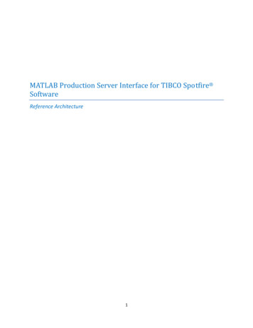
com/SpotfireWeb/ViewAnalysis.aspx?file 20Layout&configurationBlock SetPage%28pageIndex%3D0%29%3B&options 0,5-0,6-0,15-0");Enabling Javascript allows interactivity of the rendered analysis./* Enable Javascript support */WebSettings webSettings nabled(true);Finally, the application is configured to request and allow internet access. manifest . uses-permission android:name "android.permission.INTERNET" / . /manifest Our application is ready to use. In reality, the layout of a real application will be more complete andwhile it is possible to bind javascript code to the Android code, this topics are beyond the scope of this33
document. On building and running the application, we have our view rendered to the Android device.For this example, we will use a mobile phone.The custom branded application is now available as an Android application.34
Every click and interaction on the mobile device calls the MATLAB code to perform a portfoliooptimization of the data over the selected date range. In a real application, it would be necessary tooptimize the view for a mobile platform by adjusting the layout of the analysis.A similar demo would be possible for an iOS device, a detailed discussion of which is outside the scopeof this document.In conclusion, this architecture enables MATLAB powered analytics to be accessed in a reliable andscalable manner across a wide variety of platforms ranging from desktop clients, servers, web browsersand even mobile devices.35
References[1] TIBCO Spotfire - Business Intelligence Analytics Software & Data Visualization (2014, December 23rd).Retrieved from http://spotfire.tibco.com/[2] MATLAB – The language of technical computing (2014, December 23rd). Retrieved fromhttp://www.mathworks.com/products/matlab/[3] MATLAB Production Server (2014, December 23rd). Retrieved ction-server/[4] TIBCO Spotfire Data Sources (2014, December 23rd). Retrieved ata-sources[5] Portfolio Optimization (2014, December 23rd). Retrieved fromhttp://en.wikipedia.org/wiki/Portfolio optimization[6] Sharpe Ratio (2014, December 23rd). Retrieved from http://en.wikipedia.org/wiki/Sharpe ratio[7] tibbr - The social network for work (2014, January 7th). Retrieved from http://www.tibbr.com/[8] Getting started with iOS Web Apps (2015, January 7th). Retrieved erencelibrary/GettingStarted/GS iPhoneWebApp/ index.html[9] Building Web Apps in WebView (2015, January 7th). Retrieved view.html[10] Android SDK (2014, December 23rd). Retrieved from http://developer.android.com/sdk/index.html[11] Spotfire Server Environment – Clustering and Failover (2015, January 7th). Retrieved Server.aspx[12] MATLAB Production Server – Performance Optimization and Scalability (2015, January 7th).Retrieved from: -scalabilityContact InformationDave Oswill (508-647-3011)Product Marketing ManagerDave.Oswill@mathworks.comArvind Hosagrahara (310-819-3960)Principal Technical ConsultantArvind.Hosagrahara@mathworks.com36
Appendix A: Tool installationEach of the tools in the stack that comprise of the reference architecture come with its own systemrequirements and installation instructions. The coverage of all the instructions is outside the scope ofthis documents but below is a link to installation guides of each of the core components. .html) MATLAB Production Server(http://de.mathworks.com/help/pdf doc/mps/mps install.pdf) TIBCO Spotfire Server(https://docs.tibco.com/pub/spotfire server/6.5.0/TIB sfire server doc ServerInstallationManual.pdf) Installing TIBCO Web Player(https://docs.tibco.com/pub/spotfire web player/6.5.2/doc/pdf/TIB sfire webp 6.5.2 InstallationManual.pdf)An abbreviated set of notes in installing the tools to support the demonstration workflow in thisdocument can be found at ./Documentation/Installation Instructions.docx.Appendix B: Rebuilding the Spotfire ExtensionThe MathWorks.MPSExtension was built using the .NET framework 4.5 and Visual Studio 2012.The entire source code for the extension can be found inthe ./Software/Source/Spotfire/MathWorks.MPSExtension folder. The .sln file in the folder opens theextension and users can modify and build the extension using the Build- Rebuild Solution (F6) menuitem.Depending on the installation of the MATLAB Production Server product the client DLL may need to beresolved in the references. This can be done by removing the existing DLL reference and re-adding theDLL that is packaged with the installation of the MATLAB Production Server.When rebuilt, depending on the configuration, the RELEASE or DEBUG folder contains the binaries thatare used to package and create the .SPK file used for distribution. This allows the user to configure theFunctionList.xml or the ServerConfiguration.xml to point to their MPS installation.To build a new deployable Spotfire Package, start the Package Builder tool that bundles with the SpotfireSDK tools.37
First, add a Spotfire distribution by clicking on the File Add Spotfire Distribution menu item:38
To rebuild the interface, the rebuilt binaries are configured in the tool using the Add button to a newproject.Follow the wizard by clicking the Next button and creating a new module.xml file (or choosing anexisting file if you are repeating the process). Finally select the sources to bundle.39
Adjust the desired version number and finish the process.40
Right clicking on the project to build a new package file (.spk) for distribution with the Spotfire Server.The resulting SPK file can be saved and deployed to the server. Alternatively, the ‘Deploy to Server’button could be used to directly deploy the package to the Spotfire Server and make it available to allclients.41
Appendix C: Performance TipsBoth the MATLAB Production Server and TIBCO Spotfire product can be installed in clusteredconfiguration for higher performance, availability. The discussion of these configurations
This section is designed to enable the user to quickly set up a demo example integrating TIBCO Spotfire with MATLAB Production Server. Detailed information on Spotfire package deployment, troubleshooting, accessing from mobile applications etc. is available in later sections. On the machine that TIBCO Spotfire Server is running: 1.