WIXLIB

Demand ForecastingLectures 2 & 3ESD.260 Fall 2003Caplice1

AgendaThe Problem and BackgroundFour Fundamental ApproachesTime Series General ConceptsEvaluating Forecasts – How ‘good’ is it?Forecasting Methods (Stationary) Cumulative MeanNaïve ForecastMoving AverageExponential SmoothingForecasting Methods (Trends & Seasonality) OLS RegressionHolt’s MethodExponential Method for Seasonal DataWinter’s ModelOther ModelsMIT Center for Transportation & Logistics – ESD.2602 Chris Caplice, MIT2

Demand ForecastingThe problem: Generate the large number of short-term, SKUlevel, locally dis-aggregated demand forecastsrequired for production, logistics, and sales tooperate successfully.Focus on: Forecasting product demand Mature products (not new product releases) Short time horiDon (weeks, months, quarters, year) Use of models to assist in the forecast Cases where demand of items is independentMIT Center for Transportation & Logistics – ESD.2603 Chris Caplice, MIT3

Demand Forecasting – Punchline(s)Forecasting is difficult – especially for the futureForecasts are always wrongThe less aggregated, the lower the accuracyThe longer the time horizon, the lower the accuracyThe past is usually a pretty good place to startEverything exhibits seasonality of some sortA good forecast is not just a number – it shouldinclude a range, description of distribution, etc.Any analytical method should be supplemented byexternal informationA forecast for one function in a company might not beuseful to another function (Sales to Mkt to Mfg to Trans)MIT Center for Transportation & Logistics – ESD.2604 Chris Caplice, MIT4

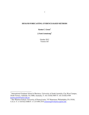
Cost of Forecasting vs InaccuracyÅ Good Region ÆÅ Overly Naïve Models ÆÅ Excessive Causal Models ÆCostTotal CostCost of ErrorsIn ForecastCost of ForecastingForecast AccuracyMIT Center for Transportation & Logistics – ESD.2605 Chris Caplice, MIT5

Four Fundamental ApproachesSubjectiveObjectiveJudgmental Causal / RelationalSales force surveysDelphi techniquesJury of experts Experimental Time SeriesCustomer surveysFocus group sessionsTest MarketingMIT Center for Transportation & Logistics – ESD.260Econometric ModelsLeading IndicatorsInput-Output Models 6“Black Box” ApproachUses past to predict thefuture Chris Caplice, MITS – used by sales/marketingO – used by prod and invAll are a search for patternJudge:Exp: new products then extrapolateCausal: sports jerseys, umbrellasTime Series: different – is not looking for cause or judgement, only repeatingpatterns6

Time Series Concepts1.2.3.4.5.6.Time Series – Regular & recurring basis to forecastStationarity – Values hover around a meanTrend – Persistent movement in one directionSeasonality – Movement periodic to calendarCycle – Periodic movement not tied to calendarPattern Noise – Predictable and random components of aTime Series forecast7. Generating Process –Equation that creates TS8. Accuracy and Bias – Closeness to actual vs Persistenttendency to over or under predict9. Fit versus Forecast – Tradeoff between accuracy to pastforecast to usefulness of predictability10. Forecast Optimality – Error is equal to the random noiseMIT Center for Transportation & Logistics – ESD.2607 Chris Caplice, MITTime Series - A set of numbers which are observed on a regular, recurring basis. Historicalobservations are known; future values must be forecasted.Stationarity - Values of a series hover or cluster around a fixed mean, or level.Trend - Values of a series show persistent movement in one direction, either up or down.Trend may be linear or non-linear.Seasonality - Values of a series move up or down on a periodic basis which can be related tothe calendar.Cycle - Values of a series move through long term upward and downward swings which arenot related to the calendar.Pattern Noise - A Time Series can be thought of as two components: Pattern, which can beused to forecast, and Noise, which is purely random and cannot be forecasted.Generating Process - The "equation" which actually creates the time series observations. Inmost real situations, the generating process is unknown and must be inferred.Accuracy and Bias - Accuracy is a measure of how closely forecasts align with observationsof the series. Bias is a persistent tendency of a forecast to over-predict or under-predict. Biasis therefore a kind of pattern which suggests that the procedure being used is inappropriate.Fit versus Forecast - A forecast model which has been "tuned" to fit a historical data set verywell will not necessarily forecast future observations more accurately. A more complicatedmodel can always be devised which will fit the old data well -- but which will probably workpoorly with new observations.Forecast Optimality - A forecast is optimal if all the actual pattern in the process has beendiscovered. As a result, all remaining forecast error is attributable to "unforecastable" noise.In more technical terms, the forecast is optimal if the mean squared forecast error equals thevariance of the noise term in the long run. Note that an optimal forecast is not necessarily a"perfect" forecast. Some forecast error is expected to occur.Some people purposely over-bias – bad idea – do not use forecasting to do inventoryplanning7

Forecast EvaluationMeasure of Accuracy / Error EstimatesNotation:Dt Demand observed in the tth periodFt Forecasted demand in the tth period at theend of the (t-1)th periodn Number of periodsMIT Center for Transportation & Logistics – ESD.2608 Chris Caplice, MITCapture the model and ignore the noise8

Accuracy and Bias Measures1. Forecast Error: et Dt - Ft2. Mean Deviation:MD n et 1tnnMAD 3. Mean Absolute Deviationn4. Mean Squared Error:MSE 5. Root Mean Squared Error:6. Mean Percent Error:7. Mean Absolute Percent Error:MIT Center for Transportation & Logistics – ESD.260tt 1n e2tt 1nnRMSE nMPE e et 1net Dt 12ttnetnMAPE 9 Dt 1tn Chris Caplice, MITMD – cancels out the over and under – good measure of bias not accuracyMAD – fixes the cancelling out, but statistical properties are not suited toprobability based dssMSE – fixes cancelling out, equivalent to variance of forecast errors, HEAVILYUSED statistically appropriate measure of forecast errorsRMSE – easier to interpret (proportionate in large data sets to MAD) MAD/RMSE SQRT(2/pi) for e NRelative metrics are weighted by the actual demandMPE – shows relative bias of forecastsMAPE – shows relative accuracyOptimal is when the MSE of forecasts - Var(e) – thus the forecsts explain all butthe noise.What is good in practice (hard to say) MAPE 10% to 15% is excellent, MAPE 20%30% is average CLASS?9

The Cumulative MeanGenerating Process:Dt L ntwhere: n t iid (µ 0 , σ2 V[n])Forecasting Model:Ft 1 (D 1 D 2 D 3 . Dt) / tMIT Center for Transportation & Logistics – ESD.26010 Chris Caplice, MITStationary model – mean does not change – pattern is a constantNot used in practice – is anything constant?Thought though is to use as large a sample siDe as possible to10

The Naïve ForecastGenerating Process:Dt Dt-1 ntwhere: n t iid (µ 0 , σ2 V[n])Forecasting Model:FMIT Center for Transportation & Logistics – ESD.260t 1 D11t Chris Caplice, MIT11

The Moving AverageGenerating Process:Dt L nDt L S nt; t tts; t twhere: n t iid (µ 0 ,σ2s V[n])Forecasting Model:Ft 1 (D t Dt-1 Dt-M 1)/Mwhere M is a parameterMIT Center for Transportation & Logistics – ESD.26012 Chris Caplice, MIT12

Moving Average ForecastsTime Series Value13012011010090292725232119171513119753180Time PeriodDtMIT Center for Transportation & Logistics – ESD.260M 213M 3M 7 Chris Caplice, MIT13

Exponential SmoothingFt 1 α Dt (1-α) FtWhere: 0 α 1An Equivalent Form:Ft 1 MIT Center for Transportation & Logistics – ESD.260Ft αet14 Chris Caplice, MIT14

Another way to think about it.Ft 1 αDt (1-α)Ft but recall that Ft αDt-1 (1-α)Ft-1Ft 1 αDt (1-α)(αDt-1 (1-α)Ft-1)Ft 1 αDt α(1-α)Dt-1 (1-α)2Ft-1Ft 1 αDt α(1-α)Dt-1 α(1-α)2Dt-2 (1-α)3Ft-3Ft 1 α(1-α)0Dt α(1-α)1Dt-1 α(1-α)2Dt-2 α(1-α)3Dt-3.MIT Center for Transportation & Logistics – ESD.26015 Chris Caplice, MIT15

Exponential SmoothingPattern of Decline in WeightEffective Weight10.8alpha .1alpha .5alpha .90.60.40.20012345Age of Data PointMIT Center for Transportation & Logistics – ESD.26016 Chris Caplice, MIT16

Forecasting Trended DataMIT Center for Transportation & Logistics – ESD.26017 Chris Caplice, MIT17

Holt's Model for Trended DataForecasting Model:Ft 1 Lt 1 Tt 1Where:Lt 1 αDt(1-α)(Lt Tt)and:Tt 1 β(Lt 1 - Lt) (1- β)TtMIT Center for Transportation & Logistics – ESD.26018 Chris Caplice, MIT18

Exponential Smoothing for Seasonal DataForecasting Model: Ft 1 Lt 1 St 1-mLt 1 α(Dt/St) (1- α) LtWhere :St 1 γ(Dt 1/Lt 1) (1- γ) St 1-m ,And :An Example where m 4, t 12:F13L13S13MIT Center for Transportation & Logistics – ESD.260 L13 S9α(D12/S12) (1- α) L12γ (D13/L13) (1- γ) S919 Chris Caplice, MIT19

MIT Center for Transportation & Logistics – ESD.260Day of /8/19999/1/1999Daily DemandSeasonal Pattern1,2001,000800600Daily Demand4002000 Chris Caplice, MIT20

Winter's Model for Trended/Seasonal DataFt 1 (Lt 1 Tt 1) St 1-mLt 1 α(Dt/St) (1- α)(Lt Tt)Tt 1 β(Lt 1 - Lt) (1- β)TtSt 1 γ(Dt 1/Lt 1) (1- γ) St 1-mMIT Center for Transportation & Logistics – ESD.26021 Chris Caplice, MIT21

Causal ApproachesEconometric Models There are underlying reasons for demandExamples:Methods: Continuous Variable Models Ordinary Least Squares (OLS) Regression Single & Multiple Variable Discrete Choice Methods Logit & Probit Models Predicting demand for making a choiceMIT Center for Transportation & Logistics – ESD.26022 Chris Caplice, MIT22

Other Issues in ForecastingData Issues: Demand Data Sales HistoryModel MonitoringBox-Jenkins ARIMA Models, etc.Focus ForecastingUse of SimulationForecasting Low Demand ItemsCollaborative Planning, Forecasting, andReplenishment (CPFR)Forecasting and Inventory ManagementMIT Center for Transportation & Logistics – ESD.26023 Chris Caplice, MIT23

Demand Forecasting - Forecasting is di Forecasts are always wrong The less aggregated, the lower the accuracy ime hori i l i include a range, description of distribution, etc. Any analytical method should be supplemented by external information useful to another function (Sales to Mkt