Transcription
International Journal of Trend in Research and Development, Volume 6(5), ISSN: 2394-9333www.ijtrd.comAircraft Demand Forecasting11,2Rajneesh Singh and 2Nikita Jain,Career Point University, Alaniya, Rajasthan, IndiaAbstract - This thesis aims to forecast aircraft demand in theaerospace and defense industry, specifically aircraft orders anddeliveries. Orders are often placed by airline companies withaircraft manufacturers, and then suddenly canceled due tochanges in plans. Therefore, at some point during the threeyear lead time, the number of orders placed and realizeddeliveries may be quite different. As a result, orders anddeliveries are very difficult to predict and are influenced bymany different factors. Among these factors are past trends,macroeconomic indicators as well as aircraft sales measures.These predictor variables were analyzed thoroughly, and thenused with time series and multiple regression forecastingmethods to develop different forecasts for quarterly and annualorders and deliveries. The relative accuracies of forecasts weremeasured and compared through the use of Theil’s U statistic.Finally, a linear program was used to aggregate multipleforecasts to develop an optimal combination of all forecasts. Inconclusion, the methods employed in this thesis are quiteeffective and produce a wholesome aggregate forecast with anerror that is generally quite low for a forecasting task aschallenging as this one.I. INTRODUCTIONIn general, forecasting techniques can be broken down intotwo different categories: qualitative or quantitative.Quantitative forecasting techniques consist of either time seriesanalysis or causal models and rely heavily on historical data.Holt’s Method, moving averages, and trend projection are justa few examples of time series techniques. Causal methodsconsist of many different regression models. To contrast,qualitative forecasting techniques are much less methodicaland rely on judgment. Some examples are the Delphi Methodand sales force composites.The goal of this thesis is to forecast aircraft demand in theaerospace and defense industry, specifically orders anddeliveries. Orders are often placed by airline companies withaircraft suppliers and then suddenly canceled due to changes inplans. Therefore, at some point during the three-year lead time,the number of orders and deliveries becomes much different.Thus, orders and deliveries are very difficult to predict, andmuch analysis must be done in order to forecast these variablesadequately.II. METHODS TO MEASURE FORECAST ACCURACYA. Time Series MethodsMethods for forecasting originated in the 1950s to 1960s andtypically did not address the random component of a timeseries. The main idea was to develop methods for predictingthe variable in question from its past data. Some of thesimplest univariate forecasting methods are the naïve nochange method, naïve change and naïve seasonal changemethod.𝒏𝒂ï𝒗𝒆 𝒏𝒐 𝒄𝒉𝒂𝒏𝒈𝒆:Ŷ𝑡 1 𝑌𝑡𝒏𝒂ï𝒗𝒆 𝒄𝒉𝒂𝒏𝒈𝒆:Ŷ𝑡 1 𝑌𝑡 (𝑌𝑡 𝑌𝑡 1 )𝒏𝒂ï𝒗𝒆 𝒔𝒆𝒂𝒔𝒐𝒏𝒂𝒍 𝒄𝒉𝒂𝒏𝒈𝒆:Ŷ𝑡 1 𝑌𝑡 (𝑌𝑡 1 𝑠 𝑌𝑡 𝑠 )IJTRD Sep – Oct 2019Available Online@www.ijtrd.comAnother method commonly used to forecast is the simplemoving-average method.In contrast to the naïve method which typically is successfulwhen the observations are relatively constant over time, themoving average method can be used to smooth data in order tosee the trend. The forecast is calculated as follows:Ŷ𝑡 1 𝑌𝑡 𝑌𝑡 1 𝑌𝑡 2 . . . . . 𝑌𝑡 (𝑘 1)𝑘Where k is the number of values in the average.Typically for quarterly data, the k value would be 4, formonthly data the k value would be 12. Typically, the larger thevalue of k, the smoother is the series.B. Regression ModelsThe first forecasting model that is of interest here is lineartrend regression. This assumes a contemporaneous relationshipbetween the dependent variable 𝑌𝑡 and the independentvariable t. α0 and α1 are parameter estimates and are estimatedby the method of least squares and ε𝑡 is a random disturbancewith zero expected value and constant variance. Parameterestimates for 𝛼0 and 𝛼1 are 𝑎0 and 𝑎1 .𝑌𝑡 𝛼0 𝛼1 𝑡 𝜀𝑡𝑌𝑡 1 𝑎0 𝑎1 (𝑡 1)C. Evaluating Forecast AccuracyThere are multiple ways to assess the accuracy of a forecast.Each technique involves comparing the forecasted value withthe realized value of a variable of interest. The amount bywhich the forecast differs from the actual value 𝑌𝑡 is theforecast error 𝑒𝑡 ,Where 𝑒𝑡 𝑌𝑡 Ŷ𝑡Four simple and commonly used measures of forecastaccuracy are presented below.Firstly, the Mean Absolute Error (MAE), also known as theMean Absolute Deviation (MAD) is as follows where n is thetotal number of observations for the period.𝒏𝒕 𝟏 𝒆𝟏MAE 𝒏Second method used often is the Mean Absolute Percent Error(MAPE). The MAPE is a modification of MAD. MAPE looksat the size of the absolute value of the error relative to theactual value itself. MAPE is presented below.MAPE 𝒏 𝒆𝒕𝒕 𝟏 𝒀𝒕𝒏 𝟏𝟎𝟎The third method for measuring error is Mean Square Error(MSE). This squares the individual errors as followsMSE 𝒏𝟐𝒕 𝟏 𝒆𝒕𝒏Finally, the Root Mean Square Error (RMSE) is simply thesquare root of the MSE. Each of these four measures can beused to determine forecast accuracy. MAPE is useful as it is40
International Journal of Trend in Research and Development, Volume 6(5), ISSN: 2394-9333www.ijtrd.comunit free. When using MSE or RMSE, having one or two largeerrors may magnify the overall measure of error. Therefore,using MAD can avoid this. When all of the errors are of thesame magnitude, RMSE and MSE are most usefulAnother, more unfamiliar measure of forecasting performanceis Theil’s U developed by Henri Theil𝑇 𝑒𝑖𝑙 ′ 𝑠 𝑈 𝑅𝑀𝑆𝐸 𝑜𝑓 𝑎𝑑𝑣𝑎𝑛𝑐𝑒 𝑎𝑝𝑝𝑟𝑜𝑐 𝑅𝑀𝑆𝐸 𝑜𝑓 𝑛𝑎ї𝑣𝑒 𝑛𝑜. 𝑐 𝑎𝑛𝑔𝑒If U 1, then the advanced approach has no value because itcannot perform as well as the naïve no change basic method.If U 1, the advanced approach has more merit. The closer Ugets to 0, the better the approach in question is. (Newbold andBos 1993)D. SeasonalitySeasonality is defined as “The estimated seasonal is that partof the series which, when extrapolated, repeats itself over anyone-year time period and averages out to zero over such a timeperiod”Combining ForecastsCombining different forecasts obtained from different but validforecasting techniques is a common practice for manyforecasters. Early researchers such as Bates, Granger,Newbold, Winkler and Makridakis presented significantevidence toward the effectiveness of combining forecasts.By combining different competing forecasts one can obtain avastly superior forecast. It is also perceivably less risky inpractice to use a combined forecast rather than selecting asingle forecastForecasting in the Airline IndustryFor lack of literature specifically in methods for forecastingaircraft demand (as top competitors such as Airbus and Boeingkeep that very private) we will focus on relevant previousresearch done on forecasting commercial airline demand.III. METHODOLOGYThe relative input variables will be discussed in greater detail,as well as their anticipated impact on the multiple regressionforecast. Additionally, this chapter will explore greateranalysis of the input variables will be explored in terms ofseasonality, volatility, correlation with one another, andultimately correlation with orders and deliveries. This analysiswill aid in understanding the underlying relationship betweenthe variables to create a more precise forecast.Long Term Interest Rate-Worldwide: Average of daily rates,measured as a percentageLong Term Interest Rate-US: Average of daily rates, measuredas a percentageJet Fuel Prices: Price per gallonCrude Oil Prices: West Texas Intermediate Price per barrel2. Aircraft Sales Figures:Aircraft Orders: Number of aircraft orderedAircraft Deliveries: Number of aircraft actually deliveredAircraft Order Cancellations: Number of aircraft cancelledAircraft Net Orders: Orders minus CancellationsInstalled Base-Active: Number of aircraft in active useRetirements: Number of aircraft retiredRevenue Passenger Mile (RPM): In Billions, measures oftraffic for airline flights; product of the number of revenuepaying passengers aboard the vehicle and the distance traveledRPM Growth: Year over year Percent changeAvailable Seat Mile (ASM): In Billions, measure of a flight'srevenue-generating abilities based upon traffic; product ofnumber of seats available and the number of miles flownASM Growth: Year over year Percent changeLoad Factor: Percentage (RPM/ASM)Operating Revenue: In millions, revenue worldwideOperating Profits: In millions, profits worldwideNet Profits: In millions, net profits worldwideIt is expected that as GDP and GDP growth increases, thenumber of orders and deliveries will increase in kind, as thenational wealth increased. Consequently, it is expected that asthe fuel price, oil price, rate of inflation and interest rate (inboth the U.S. and worldwide) increases, the number of ordersand deliveries will decrease due to the increased financialburden.Aircraft orders and deliveries are linked through aircraft ordercancellations. The nature of the aircraft sales industry is suchthat aircraft are ordered and possibly cancelled during theapproximately three-year lead time before delivery. The leadtime is not concrete and may take more or less time for anorder. Therefore, we cannot simply subtract the number ofcancellations from orders three years ago to obtain the numberof deliveries in that year. This complicates the problem further;however, we can hypothesize that an increase in the number ofcancellations will cause a decrease in the number of deliveries.A. Description of VariablesThe following lists of variables were identified by topcompetitors in the aerospace industry, such as Boeing (2014)and Airbus (2015) as potential drivers of demand. Thevariables can be grouped into two categories - globalmacroeconomic indicators and aircraft sales figures - are listedand defined below. All data is for the time period 1995 to2013, and is in quarterly and annual increments.1. Global Macroeconomic Indicators:Fig 3.1: Flow Map of the Airline IndustryGDP-Worldwide: Gross Domestic Product - The monetaryvalue of all the finished goods and services (In 2005 billion).B. Analysis of Input VariablesGDP Growth: Year over year Percent changeAn important step in the forecasting process understands theunderlying workings of each input variable. To do so, eachinput variable was graphed separately to identify any type oftrend, seasonality or cycle.Rate of Inflation Worldwide: Percentage; The rate at which thegeneral level of prices for goods and services is risingIJTRD Sep – Oct 2019Available Online@www.ijtrd.com1. Seasonality41
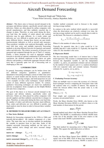
International Journal of Trend in Research and Development, Volume 6(5), ISSN: 2394-9333www.ijtrd.comThe moving average method was used to de-seasonalize thedata. It is a simple but robust tool for de-seasonalizing data andis therefore sufficient for this analysis. For the quarterly data, acentered moving average of 4 periods at a time was used toeliminate any seasonality, as the data exhibits upswings every4th quarter of each year. The idea behind a moving average isto smooth out the seasonal variation by taking a rollingaverage of the data. Then, the seasonal factors are computedby dividing the original data by the averaged data values. Next,an average is taken for each quarter’s seasonal factors toestablish one seasonal factor for each of the four quarters.Finally, the original data is divided by the correspondingseasonal factor to generate a de-seasonalized data set.Fig 3.2: Seasonality of Ordersdata. The tables below summarize the results in order fromhighest to lowest.Table 3.1 R Squared Values for Input Variables for OrdersLinear Regression for OrdersAnnual RSquaredNet Orders0.9704Operating Revenue0.6318ASM0.6165Fuel Price0.6174RPM0.6033Oil Price0.5781GDP0.5342Installed Base0.5310Load0.4958Cancellations0.3631Interest Rate US0.2950Interest Rate Worldwide0.2561Retirements0.1520GDP Growth0.1505RPM Growth0.0731ASM Growth0.0345Inflation0.0157Quarterly 02030.000Additionally, the figures presented below show an additionalview of the R squared values in decreasing order for orders anddeliveries.Fig 3.3: Seasonality of Deliveries2. VolatilityVolatility is represented as a sliding measure of the coefficientof variation (standard deviation divided by the mean). A timeframe of eight quarters was used for the quarterly data, andfour years for the annual data. The chart below represents thecoefficient of variation for each variable under four differentscenarios. The average volatility is measured for both quarterlyand annual data. In addition, the volatility of the most recentdata (2009-2013) is measured for both quarterly and annualdata.Fig 3.4: Quarterly and Annual Volatility of Input Variables3. Linear RegressionLinear regression was performed on each input variableagainst both Orders and Deliveries separately. This was doneto evaluate the predicting capacity of each variable as well asto evaluate the predicting ability of both quarterly and annualIJTRD Sep – Oct 2019Available Online@www.ijtrd.comFig 3.5. R Squared Values for OrdersBased on this analysis, deliveries seem to be overall easier topredict, as the regression, coefficients are higher than ordersfor most of the input variables. The variables RPM Growth,GDP Growth, ASM Growth were consequently eliminatedfrom further analysis due to the lack of accurate quarterly dataand insignificant correlation to the dependent variables.Fig 3.6: R Squared Values for DeliveriesIV. ANALYSIS AND RESULTSA. Forecasting Methods and ModelsKeeping the forecast simple for easy transfer to industry usewas a primary consideration. It was found that Microsoft Excel42
International Journal of Trend in Research and Development, Volume 6(5), ISSN: 2394-9333www.ijtrd.comworked well for performing most time series and regressionmethods with this data and was the preferred platform for ourindustry partners. SAS software was used for ARIMAforecasting. It was important to keep this analysis relativelyuser friendly. Excel is not only user friendly but is relativelyinexpensive. Green and Armstrong (2015) focus on similarobjectives, keeping the method simple with respect to theforecasting method and the number of input variables.2. Holt’s MethodFirst, Holt’s Method is used on the annual and quarterly data toforecast orders and deliveries. Data from 1995 to 2011 wasused to forecast for 2012 and 2013. The actual values for 2012and 2013 were then compared to the forecasted values. Thecorresponding graphs for orders are presented below.Regression analysis was recommended as a sound forecastingtechnique. In addition, it was recommended to use a weightedcombination of different forecasts. The following sectionpresents a few different methods for forecasting orders anddeliveries. Among them are Holt’s Method, Holt-Winter’sMethod, Seasonal Factor Forecasting, Lagged MultipleRegression, and ARIMA forecasting.1. Naïve No Change MethodTo provide a baseline for evaluating more advanced methods,the naïve no change method was used to forecast orders anddeliveries. The naïve no-change method simply develops aforecast for the given period (Ŷ𝑡 1 ) that is the actual valuefrom the previous period(𝑌𝑡 ). As rudimentary as this seems,this provides a baseline for which more sophisticated methodsand models should have greater accuracy.Fig 4.3: Holt's Method for Annual OrdersThe corresponding naïve no change forecasts for orders anddeliveries are presented below. As you can see, the forecast issimply the actual values shifted ahead one period.Fig 4.4: Holt's Method for Quarterly OrdersThe performance statistics are presented in the table below forboth the quarterly and annual forecasts for orders.Table 4.2: Performance Statistics for Orders Using Holt'sMethodFig 4.1: Naive No Change Forecast for OrdersQuarterlyAnnualMAPE Fit58.58%35.93%RMSE Fit321.941033.27MAPE Forecast26.02%34.10%RMSE Forecast315.61373.233. Holt-Winters MethodHolt-Winters Method was used to accommodate a potentialadditional factor of seasonality. Holt-Winters method was usedexplicitly on the quarterly data for orders and deliveries, asminor seasonality was found in both variables during theanalysis of input variables. The resulting forecasts for ordersand deliveries are presented below.Fig 4.2: Naive No Change forecast for DeliveriesThe performance statistics for orders and deliveries arepresented in the table below. Again, the Fit values are for theperiod 1995-2011 and the Forecast values are for the period of2011-2013.Table 4.1: Naive No Change Performance StatisticsOrdersDeliveriesMAPE Fit51.75%16.04%RMSE Fit327.38352.68MAPE Forecast57.84%16.21%RMSE Forecast499.96470.68IJTRD Sep – Oct 2019Available Online@www.ijtrd.comFig 4.5: Holt-Winter's Method for Quarterly Orders43
International Journal of Trend in Research and Development, Volume 6(5), ISSN: 2394-9333www.ijtrd.complot “cuts off,” it means the lags suddenly cut off after acertain number of lags, and dip lower than the 95% confidenceband. However, looking at the PACF, it seems that an ARIMA(1,1,0) model may be sufficient since the lags are notsignificant past the first one.Next, the AIC criterion will be used to decide between the twopossible models. The AIC values are presented in the tablebelow for both models.Table 4.4: AIC Values for ARIMA Models for DeliveriesFig 4.6: Holt-Winter's Method for Quarterly DeliveriesNext, the performance statistics for each forecast are presentedin the table below.Table 4.3: Performance Statistics for Orders and Deliveriesusing Holt-Winter's MethodOrdersDeliveriesMAPE Fit63.31%12.93%RMSE Fit311.4646.17MAPE Forecast29.59%9.23%4. ARIMA ForecastingIn this section, SAS software was used to analyze the seriesand ultimately generate forecasts for orders and deliveriesusing the Autoregressive Integrated Moving Average(ARIMA) model.The first step of this analysis is to identify the correct ARIMAmodel to use for each variable. SAS was used to run asequence plot of the respective variable. This aids indetermining if the series is stationary. Stationarity needs to beachieved before an ARIMA model can be used. In the SASoutput presented in the figure below, it is clear that the seriesfor deliveries is non-stationary since its autocorrelationfunction (ACF) plot decays very slowly.ModelAIC ValueARIMA (1,1,0)838.698ARIMA (0,1,2)842.576CONCLUSIONA. Overall Performance of Selected Forecasting ModelsThis thesis implemented different methods and models forforecasting aircraft orders and deliveries. Based on the resultspresented in the previous section, it is first important to notethat all forecasting techniques were deemed more accuratethan the Naïve No-Change forecast, according to Theil’s U.This indicates that each forecast is more sophisticated than themost rudimentary method and was sufficient for furtheranalysis.After aggregation with the Linear Program, it became apparentthat the Multiple Regression, Holt-Winters, and ARIMAquarterly forecasts were superior to the Holt and SeasonalFactor forecasts for both Orders and Deliveries, over theforecasting horizon of 8 quarters.The Multiple Regression model captured the past behavior ofthe economic indicators for forecasting. It was extremelyimportant to first analyze the input variables for the regressionmodel prior to forecasting, as correlations between predictorvariables needed to be identified. Highly correlated inputvariables can hinder a forecast; therefore, it was important toeliminate highly correlated input variables for the regressionanalysis.B. LimitationsFig 4.7: Initial ACF plot for DeliveriesThis thesis focused on a forecasting horizon of two years, oreight quarters which maintained the relative accuracy of theforecasts given the respective models. However, proceedingfurther out to a longer forecasting horizon would undoubtedlynegatively impact the forecasting accuracy as a whole.Therefore, the aggregate forecasting methods employed in thisthesis are limited. More robust machine learning methodscould be considered to forecast a longer horizon and areexpected to improve accuracy.References[1][2][3]Fig 4.8: ACF and PACF plots for Differenced DeliveriesSince the data is non-stationary, it was first differenced in SASby taking the logarithm of the data. The figure above displaysthe autocorrelation function (ACF) plot as well as the partialautocorrelation plot (PACF) for the differenced series. Theautocorrelation plot of the differenced series suggests that theseries is now stationary. The ACF plot cuts off after the 3rd lag(above the 95% confidence level), therefore this implies thatan ARIMA (0,1,2) model could be used. Essentially, when aIJTRD Sep – Oct 2019Available Online@www.ijtrd.com[4][5][6][7][8]Green, K.C., Armstrong, J.C., “Simple Forecasting: Avoid Tearsbefore Bedtime”, 2015.Ho, K. K., “Demand forecasting for aircraft engine aftermarket”,2008.Yu, G. (Ed.), “Operations research in the airline industry” (Vol. 9),2012.Liehr, M., Größler, A., Klein, M., & Milling, P. M. “Cycles in thesky: understanding and managing business cycles in the airlinemarket”, 2001Hibon, M., & Evgeniou, T. “To combine or not to combine: selectingamong forecasts and their combinations”, 2005.Fang, Y. “Forecasting combination and encompassing tests”, 2003.Enders, Walter. “Applied Econometric Time Series”, 2004Carson, R. T. “Forecasting (aggregate) demand for US commercialair travel”, 2011.44
Aircraft Demand Forecasting 1Rajneesh Singh and 2Nikita Jain, 1,2Career Point University, Alaniya, Rajasthan, India . forecasting techniques is a common practice for many forecasters. Early researchers such as Bates, Granger, Newbold, Winkler and Makridakis presented significant evidence toward the effectiveness of combining forecasts. .