Transcription
Semi-supervised Data Clustering with CoupledNon-negative Matrix Factorization: Sub-categoryDiscovery of Noun Phrases in NELL’s KnowledgeBaseTom MitchellMachine Learning DepartmentCarnegie Mellon Universitytom.mitchell@cs.cmu.eduChunlei LiuMachine Learning DepartmentDepartment of PhysicsCarnegie Mellon Universitychl56@andrew.cmu.eduAbstractThe standard non-negative matrix factorization (NMF) is a popular method to obtain low-rank approximation of a non-negative matrix, which is also powerful forclustering and classification in machine learning. In NMF each data sample isrepresented by a vector of features of the same dimension. In practice, we oftenhave good side information for a subset of data samples. These side informationmight be binary vectors that indicate human provided class labels, or generic vectors in a different feature space. In this paper we propose the coupled non-negativematrix factorization (CNMF) method to automatically incorporate the side information of a subset of data. In CNMF, the matrix for data samples with or withoutside information in the original feature space and the matrix for data samples withside information in the new feature space are coupled together and iteratively optimized. Because of different qualities of the side information, a trade-off parameteris introduced to determine the importance of the side information, and we give across validation method to choose its value. The time complexity of the CNMFmethod could be several times bigger than the original NMF method, but still inthe same order. As an example of implementing the CNMF method, we lookinto the knowledge base of the CMU Never-Ending Language Learning (NELL)project and find sub-categories of noun phrases.1IntroductionApplication of clustering with multi-dimensional data is important in many fields, including information retrieval, text mining, image grouping and medical diagnosis. For many situations, we couldm ndefine non-negative measurements of different features as data set X {x1 , ., xn } R ,where each of the n samples is a m-dimensional non-negative feature vector. The standard clustering is usually unsupervised, where we hope to find the natural grouping of data samples based onmeasured or perceived similarities in the feature space. We explore methods to improve the clustering performance based on good side information on a subset of data samples, which is affordablein many cases. The side information could be class labels provided by domain experts, or moreexpensive and better measurements in a different feature space. As long as the side informationis clean and allows easy clustering of the subset of data samples, the original clustering becomessemi-supervised and the performance can be improved. The side information can be represented bym0 n0a matrix as Y {y1 , .yn0 } R , where n0 n and each data sample is a m0 -dimensionalnon-negative feature vector. For example, if the side information are class labels, each data sample1
in Y will a binary vector with the jth entry being 1 and the remaining elements being 0 if it is fromclass j.As a case study, we cluster noun phrases from the knowledge base of the Never-Ending LanguageLearning (NELL) project at CMU [1]. Since it was launched in January 2010, NELL has extractedmillions of noun phrases and relation instances by reading the web. There are currently more thanone hundred top noun categories in NELL’s knowledge base, such as Species, Chemical,Religion, Economic Sector, and Emotion. In the very beginning, the initial ontologyof noun categories and relations are given. As times goes, NELL populates the noun categories andrelations by learning new instances. For each main noun category, as there are more and more nounphrases learned, it is useful to discover good sub-categories with clustering methods, such that newnoun phrases can be better learned and classified. For example, the Animal category has more thantwenty thousand instances currently. In Tab. 1 we also show some noun phrase instances under the“movie” and “plant” category in NELL’s knowledge base.The input data set X for noun phrases from NELL is the co-occurrence matrix between noun phraseand context from input sentences. Both the noun phrase and context are defined using part-ofspeech tag sequences. Each context can be viewed as a feature of the noun phrases, and the cooccurrence statistics is the measurement. The initial size of the context feature space is enormous,so in order to decrease the dimension and reduce computational time later, we only keep contextsthat have co-occurrence bigger than a defined threshold. Further feature selections can also beapplied, such as choosing the top ranked context features according to the co-occurrence with thenoun phrases. Side information on part of the noun phrases can be obtained using relation instancesbetween noun categories from NELL. For example, there are about two thousand instances in therelation (arg1) animal is type of animal (arg2), where both arguments are from theanimal category. Instances in this relation category, e.g., (robin) is type of (bird), havesubset/superset relations, as the first argument is a member of the second argument. Representingall the first arguments as columns and all the second arguments as features in rows, we can build theside information matrix Y , where each cell is either zero or one.CategoryMoviePlantNoun phrase instancesaliens; an american in paris; beowulf;big lebowski; boogie nights; close encounters;collateral; dick tracy; die hard;doctor zhivago; empire strikes back;ferris bueller s day off; fight club;forrest gump; goblet of fire; godzilla;goodfellas; good will hunting; hamlet hook; .spruces; alders; algae; allium; annuals;apple tree; apple trees; aquatic plants;aquatic weeds; ash; ash trees; aspen; aspens;asters; azalea; azaleas; bamboo; banana trees;basswood; bean; .Table 1: Examples of categories and noun phrases in NELL’s knowledge base.In the following sections, we first describe several traditional clustering methods. We then focus onthe clustering method based on NMF and how to improve it with CNMF, and we demonstrate theperformance of CNMF through studies of synthesized data. In the following experiment section,we first implement several feature selection methods, then show the results of using traditionalclustering methods, NMF and CNMF, separately.2Traditional Clustering MethodsGeneral clustering methods can be divided into two main categories: hierarchical and partitional. Ina hierarchical algorithm, a dendrogram is created to represent the similarity levels at which groupings change. The most popular hierarchical algorithms include the single-link [2] and completelink [3] algorithms. For the partitional clustering algorithm, on the contrary, a single partition ofthe data instead of a clustering structure is obtained. Since hierarchical algorithms are usually com2
putationally prohibitive, partitional methods have the advantages in application that involve largedata.The most frequently used criterion function in partitional clustering is the squared error criterion.This criterion tends to work well if the data is isolated and compact. The K-means algorithm [4] isthe simplest algorithm that uses this squared error metric. We can also employ other distance metrics such as the cosine distance for the K-means, which might work better for certain data. Anothercommonly used partitional methods is the mixture model based algorithms. The underlying assumption is that the data to be clustered are drawn from several different distributions corresponding todifferent clusters. The goal of the algorithm is to identify the parameters for each distribution. Tocluster data that has no real labels known, the Expectation Maximization (EM) algorithms can beapplied [5].2.1K-means Algorithmm nGiven a set of observations X {x1 , ., xn } R , where each observation is a mdimensional vector, K-means clustering algorithm partitions the n observations into K sets S {S1 , S2 , ., SK }, such that the within-cluster sum of squared distances to the centroid is minimized:arg minSK XX Xj µi 2 ,(1)i 1 Xj Siwhere we have used the Euclidean distance, and µi is the mean of points in cluster Si . To find theoptimal cluster assignments, the K-means algorithm uses an iterative refinement technique. First,the data points are given some initial cluster assignments (e.g., random initialization). Then thealgorithm proceeds by alternating between the following two steps until assignments of clusters nolonger change: Assignment step: assign each data point to the cluster whose mean is closest to it; Update step: re-calculate the mean of each cluster as the centroid of that cluster.The original K-means algorithm described here is known to find local optima only. To overcomethis problem, we actually use the K-means algorithm which aims at a better initialization [6] toavoid being stuck at a local optima. The specific algorithm is as follows: The first cluster center is chosen uniformly at random from among all the data points. For each data point x, compute the distance D(x) between x and the nearest center that hasbeen chosen. Choose one new data point as a new center according to the probability that is proportionalto D2 (x). Repeat the second and third steps until all the needed centers have been chosen. With all the initial cluster centers chosen we proceed using the standard K-means clustering.2.2Multinomial Mixture ModelWe use the multinomial mixture model with naive Bayes assumption to model the data we have. Inthe frame work of supervised learning, where the true cluster label of each instance is known, it iseasy to estimate the parameters. A mixture model is a linear combination of models as:XP (X) P (Z)P (X Z)Zwhere Z identifies the mixture component. P (Z) is the probability of generating component Z, andP (X Z) is the distribution associated with the mixture component Z. In this project, we assumeP (X Z) is a multinomial distribution, and Z 1, ., L are the cluster labels. After we learn P (Z)and P (X Z), we can compute the cluster probabilities for each data item Xi as :P (Z Zi X Xi ) P (Z Zi )P (X Xi Z Zi ).3
We then assign data Xi the label as argmax P (Z Zi X Xi ). In order to apply the mixturemodel, we need to learn the parameters associated with probability density functions first. Form nX {x1 , ., xn } R the row index is j {1, ., m} for each data sample Xi . The numberof times row j co-occurs with Xi is Nj (Xi ). The parameters and probability density functions arelinked through:P (Zi k) φkP (Xi,j Zi k) θk,jN (Xi )jP (Xi , Zi k) φk ΠLk 1 θk,jThe sufficient statistics for estimating parameters in the multinomial mixture using the maximumlikelihood method is as follows:Pn nk Pi 1 I(Zi , k), i.e., number of times clusters k is seen.n nk,j i 1 Nj (Xi )I(Zi , k), i.e., number of times context j is seen in cluster k.If the cluster label of each Xi is known, the maximum likelihood gives estimates as:nkφk nnk,jθk,j Pn0j 0 1 nk,j(2)In our case, since we do not know the true label of each animal instance, we cannot estimate theparameters with the training data. However, we can still obtain estimations using the EM algorithmsas the following: Guess the initial values φ(0) and θ(0) Repeat the following, for iterations t 1,2,.:– E-step: calculate the expected values of sufficient statistics:E[nk ] nXPφ(t 1) ,θ(t 1) (Zi k Xi )(3)i 1E[nk,j ] nXNj (Xi )Pφ(t 1) ,θ(t 1) (Zi k Xi )i 1– M-step: update the parameters based on sufficient statisticsE[nk ]nE[nk,j ] Pn0j 0 1 E[nk,j ](t)φk (t)θk,j(4) after convergence of previous step, assign label to each data Xi as argmax P (Z Zi X Xi ).2.3Clustering Through Dimension ReductionClustering algorithms that are based on distance measure are often not effective for data with highdimensions, as distance between nearest points in high dimension is not different from that of otherpoints [7]. On the other hand, in practice, high dimensional data usually have much lower intrinsicdimension which makes clustering possible and reduces computational cost. Methods such as thePrinciple component analysis (PCA) construct a linear combination of low dimensional vectors thatcan best describe the variance of the original data [8]. There are also non-linear methods such asthe Multidimensional Scaling (MDS) [9] and the Spectral Clustering algorithm [10]. In the MDSmethod, the original high dimensional data are projected into a low dimensional structure whilemaintaining the proximity information. For the spectral clustering algorithm, the similarity matrixbetween different points in the data are constructed, and the clustering algorithm partitions the datainto different subsets by optimizing certain criterion functions.4
3Clustering Method with Matrix Factorization and Related WorkNon-negative matrix factorization (NMF) is similar to the spectral clustering algorithm, and hasbeen shown to be very useful in presenting non-negative data with intuitive basis vectors [11]. Withthe NMF method, we can obtain a lower rank-k approximation by factorizing the data matrix X m nm kk nR into two non-negative factor matrix W R and H R by minimizing the followingcost function:1min f (W, H) X W H 2F ,(5)W 0,H 02where F stands for Frobenius norm, W is referred as the basis matrix and H is called as encodingmatrix. Given the rank k, the NMF aims at finding the best basis axis to project the original dataonto a k-dimensional space. Columns of the basis matrix W gives the basis vectors, and columnsof the encoding matrix H gives the membership of each new dimension for the data points. Theoptimization problem shown in Eqn. 5 is not convex, so it is hard to find the global minimum.However if W satisfies the separability condition, algorithms for exact solution with polynomialrunning time have been given [12]. In many cases finding local minimum is still useful. Variousalgorithms have been invented to find factor matrix W and H, including multiplicative update rule[13] and several algorithms based on alternating non-negative least squares, such as the projectedgradient descent methods [14], the active-set method [15] and the block principal pivoting method[16].The NMF method has been successfully used in clustering problems as in [17]. In the NMF space,each basis axis can be related to a cluster. Clustering the data points is equivalent as finding the axiswith which the data point has the largest projection value in the encoding matrix H. We can alsoview the NMF as a dimension reduction method and further apply traditional clustering methodssuch as K-means on the column vectors in H.Several semi-supervised NMF methods have been developed to incorporate prior knowledge andto improve the clustering performance [18],[19],[20]. Our proposed coupled non-negative matrixfactorization (CNMF) method is distinguished from these existing work in several ways: While some methods use pairwise must-link or cannot-link constraints [18],[19], and othermethods exploit class labels on a few data samples [20], our CNMF method assumes sideinformation in a more general feature space. The pairwise constraints or class labels can betreated as a special case of feature vectors in CNMF. Notice that these constraints are softconstraints in CNMF, and the strength can be controlled by a trade-off parameter. Compared to method used in [20], no extra weight matrix is needed in CNMF to distinguish data samples which have side information available or unavailable. Instead, CNMFemploys a sum of three residuals to mathematically and intuitively couple the data matrixwithout side information, the data matrix with side information and the side informationmatrix together. We develop updates for the projected gradient method as in [14], which are different fromalgorithms used in other methods [18],[19],[20] such as multiplicative updated. Similar to the method in [20], we introduce a trade-off parameter to determine the influenceof the side information matrix, but we also introduce a cross validation method to choosethe size of the parameter.4Clustering Method with Coupled Non-negative Matrix FactorizationFirst we notice that the side information matrix Y can be separately factorized as the data matrix Xin Eqn. 5. In this case, we optimize the following objective function:1minf (WY , HY ) Y WY HY 2F .(6)WY 0,HY 02Since X and Y share a common subset of data samples, we divide X into two parts X1 and X2 ,where X1 and X2 has the same number of rows (features) but different number of columns (datapoints). Columns of X2 represent the same subset of data samples as in Y , while columns of X1represent all the remaining data samples. Thus factorizing X is equivalently as optimizing:11minf (WX , H1 , H2 ) X1 WX H1 2F X2 WX H2 2F ,(7)WX 0,H1 0,H2 0225
where we factor X1 and X2 onto the same basis matrix WX but different encoding matrices H1 andH2 . We further notice that matrix X2 and Y represent the same subset of data samples in differentfeature spaces, but they are related by having the same encoding matrix with HY H2 . Thus weobtain the final coupled optimization objective function as:minWX 0,WY 0,H1 0,H2 0f (WX , WY , H1 , H2 )(8)111 X1 WX H1 2F X2 WX H2 2F Y WY H2 2F ,222where all the factor matrices are coupled in the same function such that good side information leadsto good encoding matrix H2 for data samples with side information, good H2 matrix then helps tofind good basis matrix WX , and eventually good WX results in good encoding matrix H1 for theremaining data samples. After the solutions are obtained, we concatenate on H1 and H2 to get theencoding matrix for all data samples. When optimizing the objective function in Eqn. 8, in order to balance different terms, it is better tofirst normalize X1 , X2 and Y by column with some normalization method such as L2-norm. Considering different qualities of the side information in Y , we can also introduce a trade-off parameterλ:minWX 0,WY 0,H1 0,H2 0 f (WX , WY , H1 , H2 )(9)11λ X1 WX H1 2F X2 WX H2 2F Y WY H2 2F ,222where if λ 0, the CNMF is same as the original NMF of X without any side information, while ifλ gets bigger, the role of side information becomes more important in the CNMF.Like the original NMF, the CNMF problem shown in Eqn. 9 is a non-convex optimization problem.Here we apply the projected gradient algorithm based on ANLS as shown in Alg. 1 to find a localminimum. In order to solve the subproblems as in Eqn. 11 14, we need to calculate the gradientand Hessian matrix for each factor matrix. One difference from the method in [9] is that we haveH2 coupled in two terms, where the gradient for H2 is:TT f (H2 ) (WXWX )H2 WXX2 λ((WYT WY )H2 WYT Y ),TWX λWYT WY . To checkand the Hessian matrix is block diagonal with each block equals WXthe convergence of the algorithm, we compare the function value at each iteration to the value fromthe previous iteration. The convergence is achieved if the change is smaller than a defined threshold(e.g., 10 6 ). The time complexity of this algorithm is similar to the original projected gradient algorithm. For each outer iteration, the original NMF with projected gradient algorithm need O(tmk 2 )to minimize H and O(tnk 2 ) to minimize W , where t is the number of inner iterations. In CNMF,there are more terms to minimize for each outer iteration, so the cost could be several times biggerthan the NMF without the side information.The size of parameter λ in Eqn. 9 can be chosen with cross validation methods using some hold-outdata. After the basis matrix WX is obtained by factorizing the matrix X, we use it to factorize thehold-out data by optimizing the following objective function:1 Xhold WX Hhold 2F ,Hhold 0 2min(10)where Xhold is the matrix for the hold-out data, and Hhold gives us the memberships of the holdout data on different basis axis. The optimized function value of the hold-out data can be used tocompare performances of factorizing X with different size of λ, where smaller function value meansbetter factorization.5Studies with Synthesized DataTo simulate the data matrix X, we generate 600 data samples with 2000 features from 10 clustersusing the following procedure. Every consecutive 60 samples are generated from the same cluster.For each cluster, we randomly pick 300 out of 2000 features. Then for each sample in the same6
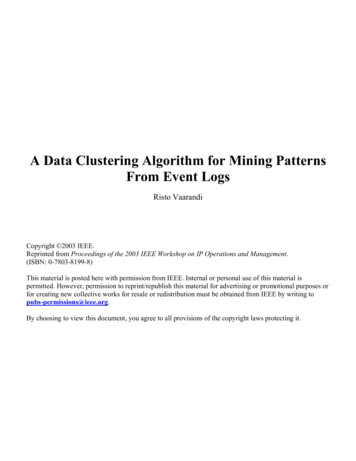
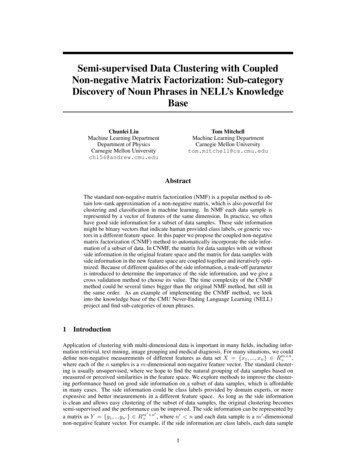
Algorithm 1 Alternating nonnegative least squares for CNMF1Initialize: WX 0, WY1 0, H11 0, H21 0repeatfor k 1 to 1, 2, . doWYk 1H1k 1H2k 1k 1WX kargminWY 0 f (WX, H1k , WY , H2k )(11) kargminH1 0 f (WX, H1 , WYk 1 , H2k )kargminH2 0 f (WX, H1k 1 , WYk 1 , H2 )argminWX 0 f (WX , H1k 1 , WYk 1 , H2k 1 )(12) (13)(14)end foruntil convergencecluster we randomly pick half of the 300 cluster features and assign them random values between 1and 50, and assign 0 to all the remaining features. After the data are generated, we add a uniformlydistributed random number between 1 and 100 to all feature values of all the data as noise. Wesimulate the side information matrix in three different ways: (1) We randomly choose 6 data samplesfrom each cluster and define a new feature space of dimension 10. For all the 6 data samples comingfrom the same cluster, we set the jth feature value to be 1 and 0 for the remaining features if the datasample is from the jth cluster. This corresponds to giving the class labels to part of the data samples.We denote this side information matrix as Y1 . (2) We randomly choose 6 data samples from eachcluster and define a new feature space of dimension 300. For all the 6 data samples coming from thesame cluster, we randomly select 30 features and set their value to be 1 and 0 for all the remainingfeatures. This corresponds to good measurements of part of the data samples in a new feature space.We denote this side information matrix as Y2 . (3) We randomly choose 6 data samples from eachcluster and define a new feature space with dimension 300. For each data sample, we set all of theirfeature values to be random numbers between 0 and 1. This corresponds to noisy and completelyuninformative side information. We denote this side information matrix as Y3 .In order to find a reasonable size of λ in Eqn. 9, we take 100 data samples as the hold-out data bychoosing 10 samples from each cluster. Data samples which have side information are excludedwhen generating the hold-out data. The remaining 500 data samples are put into matrix X and wealso have side information on 60 data samples. For each type of side information encoded in Y1 , Y2and Y3 , we vary the size of λ and apply algorithm 1 to optimize the objective function in Eqn. 9.With the factor matrices obtained, we then optimize the objective function in Eqn. 10 using thehold-out data set. The function value of the hold-out data set versus λ value are shown on the left ofFig. 1. According to the results, using good side information in Y1 or Y2 leads to better factorizationof the hold-out data set as the value of λ increases. On the other hand, if the side information israndom noise and thus useless, the factorization could get worse as we increase the value of λ. Thebenefits of using good side information in the CNMF can also be seen by visualizing the encodingmatrix H. In Fig. 2, we show the transpose of the H matrix with Y2 for the first six λ values. As thevalue of λ increase from 10 4 to 0.1, the 10 clusters can be seen more and more clearly.In previous situations, we have side information for data samples from all the 10 clusters. In practice,we might only have side information for data samples from part of the clusters. We check theperformance of the CNMF by simulating matrix Y from only 5 clusters. Specifically, we set up Yusing the second method as previously discussed, but with side information for only 30 data samplesfrom 5 clusters only ( 6 data samples from each cluster). We also take 100 randomly chosen datasamples from each cluster as the hold-out data set, and use the remaining 500 data samples andside information on 30 data samples to implement the CNMF. With the results, we optimize theobjective function in Eqn. 10 using the hold-out data set. The function value versus different size ofλ is shown on the right of Fig. 1, where we can see that the factorization also gets better as the valueof λ increases.7
Figure 1: (left) Value of the objective function from Eqn. 10 versus λ with side information fromall the 10 clusters, which is calculated on a hold out data set independent of the training set. (right)Value of the objective function as in Eqn. 10 versus λ using a hold out data set with side informationfrom half of the 10 clusters .Figure 2: HT (encoding matrix) of 500 training samples for different λ values, with good sideinformation from Y2 .6ExperimentsWe look into NELL’s knowledge base and use the co-occurrence matrix between noun phrase andcontext as the input data. As an example, we obtain the co-occurrence matrix for the Animalcategory which has about 20 thousand animal instances and about 5 million context features. Wefurther choose the top 600 popular animal instances to serve as our training data set, where thepopularity is ranked according to their total co-occurrences with all the context features.In the following sections, we first describe different ways of selecting features. We then apply theKmeans and EM algorithms to cluster the training data set. In order to obtain side information and8
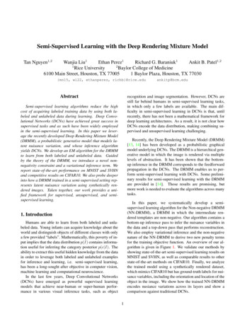
improve the cluster results, we look into the relation instances involving animal instances and applythe CNMF method.6.1Feature selectionContexts of the co-occurrence matrix can be viewed as features of the animal instances. For the 600training data, the initial dimension of the feature space is about 379 thousands. It is computationallyexpensive to perform the following clustering analysis, and the result might be degraded as well. Inorder to improve the clustering result and reduce computational burden, we apply different featureselection methods.The first feature selection method is to rank contexts according to their total co-occurrences with allthe animal instances. We then choose the contexts that have high ranks in the list as the features. Asan example, we show the top 20 and bottom 20 contexts in Tab. 2.Ranktop 20bottom 20Contextsnumber of ; species of ; you have ;’s life;’s books; group of ; needs of ; care of ;is in;are in;thousands of ; I was ;variety of ;living in;’s name; kind of; types of ; lot of ; parents of ; lives of.likely consume ;has product development;’s lead drug; Iowa ; started ; care havemade ; Fables From ; Unnatural History of ;’s Pizzeria; saltmanager , has been with ;deposits at ; deposits at ; Alumni AssociationDistinguished ; Association ?s Distinguished;moving hundreds; paste recipe for ;awarded since; Other companies using ; salesof western ; jet thompson ; Council features .Table 2: Examples of contexts ranked according to their total co-occurrence with all the animals.As we can see from the results, it is easy to see that highly ranked contexts co-occur frequently withanimal instances, while lowly ranked contexts does not have any meaningful relationship with animal instances. We further check some statistics associated with the resulting co-occurrence matrix.Taking the top 2,000 contexts as an example, the co-occurrence matrix has a dimension of 2000 by600. In Fig. 3, we show the number of contexts out of the 2000 contexts each animal co-occur with,and the average number of co-occurrence for each animal with these contexts. On average, eachanimal instance co-occurs with 704 contexts with a mean co-occurrence frequency of 17.In the first method, although highly ranked contexts based on total co-occurrence with all the animalinstances are good for the whole category, they might be not very powerful to distinguish differentsub-categories. An an improvement, we first choose a much larger subset of contexts with the firstmethod, then we apply a different method to refine it. Here we propose the second method following[21] that defines the variance quality for the jth context as the following:"m#2m1 X 21 X 2q(j) f f,(15)m i 1 ij m2 i 1 ijwhere m is the total number of animal instances (600 in this case), and fij is the co-occurrence ofbetween animal instance i and context j. The variance quality tells us the variances of co-occurrencebetween each context and all the animals. Intuitively, the larger the value of the variance is, thestronger distinction power the context has. We choose the top 100 thousands contexts using the firstmethod, then we calculate the variance quality for all these 100 thousands contexts and rank themaccording to the variance quality. Here we list the top 20 and bottom 20 contexts in Tab. 3.We further check the resulting co-occurrence matrix. Taking the top 2,000 contexts as an example,where the dimension of the co-occurrence matrix is 2000 by 600. In Fig. 4, we show the number9
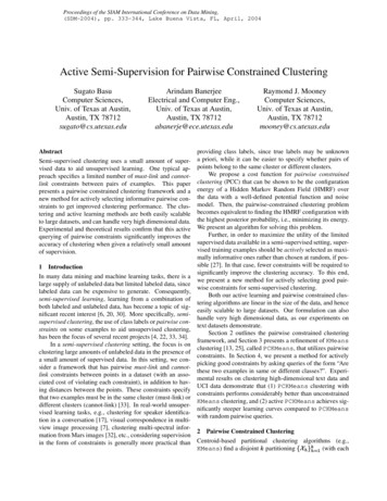
Figure 3: Ranking contexts according to the total co-occurrences with all animal: (left) Numberof contexts out of 2000 top ranked contexts each animal instance co-occurs with, (right) averagenumber of co-occurrence per context for each animal. In both plots, the animal instances are sortedaccording to the total co-occurrences with all the contexts.Ranktop 20bottom 20Contextsnumber of ;’s books; I was ; needs of ;’s Hospital;’s life; families with ; parentsof ; Son of ; click of ; you have ; lives of; reach of ;’s book;’s education; care of;’s literature;’s share;’s hand;’sname.are well known in;were moving into; sameare as large; creature resemblingleague as ;;still survive in; it did n’t take longfilling the air; It was filled withfor ;; Today , with ; complete lack of ; forestsma
Tom Mitchell Machine Learning Department Carnegie Mellon University tom.mitchell@cs.cmu.edu Abstract The standard non-negative matrix factorization (NMF) is a popular method to ob-tain low-rank approximation of a non-negative matrix, which is also powerful for clustering and classification in machine learning. In NMF each data sample is