TODL Semi-Supervised Learning - WordPress PDF Free Download

2y ago

39 Views

1 Downloads

1.22 MB

12 Pages

Report/dmca

Download PDF

Transcription

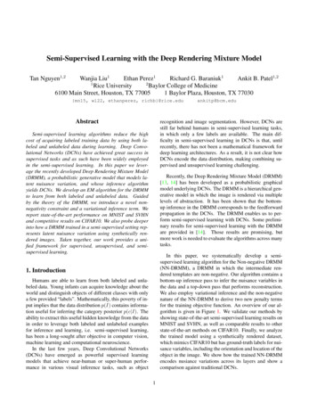
Semi-Supervised Learning with the Deep Rendering Mixture ModelTan Nguyen1,2Wanjia Liu1Ethan Perez1Richard G. Baraniuk1Ankit B. Patel1,212Rice UniversityBaylor College of Medicine6100 Main Street, Houston, TX 770051 Baylor Plaza, Houston, TX 77030{mn15, wl22, ethanperez, richb}@rice.eduAbstractankitp@bcm.edurecognition and image segmentation. However, DCNs arestill far behind humans in semi-supervised learning tasks,in which only a few labels are available. The main difficulty in semi-supervised learning in DCNs is that, untilrecently, there has not been a mathematical framework fordeep learning architectures. As a result, it is not clear howDCNs encode the data distribution, making combining supervised and unsupervised learning challenging.Semi-supervised learning algorithms reduce the highcost of acquiring labeled training data by using both labeled and unlabeled data during learning. Deep Convolutional Networks (DCNs) have achieved great success insupervised tasks and as such have been widely employedin the semi-supervised learning. In this paper we leverage the recently developed Deep Rendering Mixture Model(DRMM), a probabilistic generative model that models latent nuisance variation, and whose inference algorithmyields DCNs. We develop an EM algorithm for the DRMMto learn from both labeled and unlabeled data. Guidedby the theory of the DRMM, we introduce a novel nonnegativity constraint and a variational inference term. Wereport state-of-the-art performance on MNIST and SVHNand competitive results on CIFAR10. We also probe deeperinto how a DRMM trained in a semi-supervised setting represents latent nuisance variation using synthetically rendered images. Taken together, our work provides a unified framework for supervised, unsupervised, and semisupervised learning.Recently, the Deep Rendering Mixture Model (DRMM)[13, 14] has been developed as a probabilistic graphicalmodel underlying DCNs. The DRMM is a hierarchical generative model in which the image is rendered via multiplelevels of abstraction. It has been shown that the bottomup inference in the DRMM corresponds to the feedforwardpropagation in the DCNs. The DRMM enables us to perform semi-supervised learning with DCNs. Some preliminary results for semi-supervised learning with the DRMMare provided in [14]. Those results are promising, butmore work is needed to evaluate the algorithms across manytasks.In this paper, we systematically develop a semisupervised learning algorithm for the Non-negative DRMM(NN-DRMM), a DRMM in which the intermediate rendered templates are non-negative. Our algorithm contains abottom-up inference pass to infer the nuisance variables inthe data and a top-down pass that performs reconstruction.We also employ variational inference and the non-negativenature of the NN-DRMM to derive two new penalty termsfor the training objective function. An overview of our algorithm is given in Figure 1. We validate our methods byshowing state-of-the-art semi-supervised learning results onMNIST and SVHN, as well as comparable results to otherstate-of-the-art methods on CIFAR10. Finally, we analyzethe trained model using a synthetically rendered dataset,which mimics CIFAR10 but has ground-truth labels for nuisance variables, including the orientation and location of theobject in the image. We show how the trained NN-DRMMencodes nusiance variations across its layers and show acomparison against traditional DCNs.1. IntroductionHumans are able to learn from both labeled and unlabeled data. Young infants can acquire knowledge about theworld and distinguish objects of different classes with onlya few provided “labels”. Mathematically, this poverty of input implies that the data distribution p(I) contains information useful for inferring the category posterior p(c I). Theability to extract this useful hidden knowledge from the datain order to leverage both labeled and unlabeled examplesfor inference and learning, i.e. semi-supervised learning,has been a long-sought after objective in computer vision,machine learning and computational neuroscience.In the last few years, Deep Convolutional Networks(DCNs) have emerged as powerful supervised learningmodels that achieve near-human or super-human performance in various visual inference tasks, such as object1

AB𝐸 : Top-DownReconstructionCClassification Cross Entropy, ℒ𝐻K-L Distance, ℒ𝐾𝐿𝜇𝑐13Update 𝜇𝑐42ONOFFΛ𝑔(𝐿)Total Loss, ℒUpdate Λ𝑔(ℓ)1324Λ𝑔(ℓ)RenderingNon-Negativity Constraint, ℒ𝑁𝑁Reconstruction Error, ℒ𝑅𝐶Λ𝑔(1)Noise𝐸 : Bottom-UpInferenceFigure 1: Semi-supervised learning for Deep Rendering Mixture Model (DRMM) (A) Computation flow for semi-supervised DRMMloss function and its components. Dashed arrows indicate parameter update. (B) The Deep Rendering Mixture Model (DRMM). Alldependence on pixel location x has been suppressed for clarity. (C) DRMM generative model: a single super pixel x( ) at level (green,upper) renders down to a 3 3 image patch at level 1 (green, lower), whose location is specified by g ( ) (light blue). (C) shows onlythe transformation from level of the hierarchy of abstraction to level 1.2. Related WorkWe focus our review on semi-supervised methods thatemploy neural network structures and divide them into different types.Autoencoder-based Architectures: Many early works insemi-supevised learning for neural networks are built uponautoencoders [1]. In autoencoders, the images are firstprojected onto a low-dimensional manifold via an encodingneural network and then reconstructed using a decodingneural network. The model is learned by minimizing thereconstruction error. This method is able to learn fromunlabeled data and can be combined with traditional neuralnetworks to perform semi-supervised learning. In thisline of work are the Contractive Autoencoder [16], theManifold Tangent Classifier, the Pseudo-label DenoisingAuto Encoder [9], the Winner-Take-All Autoencoders[11], and the Stacked What-Where Autoencoder [20].These architectures perform well when there are enoughlabels in the dataset but fail when the number of labelsis reduced since the data distribution is not taken intoaccount. Recently, the Ladder Network [15] was developedto overcome this shortcoming. The Ladder Networkapproximates a deep factor analyzer where each layer in themodel is a factor analyzer. Deep neural networks are thenused to do approximate bottom-up and top-down inference.Deep Generative Models: Another line of work in semisupervised learning is to use neural networks to estimatethe parameters of a probabilistic graphical model. Thisapproach is applied when the inference in the graphicalmodel is hard to derive or when the exact inference iscomputationally intractable. The Deep Generative Modelfamily is in this line of work [7, 10].Both Ladder Networks and Deep Generative Modelsyield good semi-supervised learning performance on

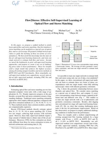
Q(L)benchmarks.They are complementary to our semisupervised learning on DRMM. However, our method isdifferent from these approaches in that the DRMM is thegraphical model underlying DCNs, and we theoreticallyderive our semi-supervised learning algorithm as a properprobabilistic inference against this graphical model.Λg( ) µc(L) represents the sequence of local nuisancetransformations that partially render finer-scale details aswe move from abstract to concrete. Note that the factorizedstructure of the DRMM results in an exponential reductionin the number of free parameters. This enables efficientinference, learning, and better generalization.Generative Adversarial Networks (GANs): In the lastfew years a variety of GANs have achieved promising results in semi-supervised learning on different benchmarks,including MNIST, SVHN and CIFAR10. These models alsogenerate good-looking images of natural objects. In GANs,two neural networks play a minimax game. One generates images, and the other classifies images. The objectivefunction is the game’s Nash equilibrium, which is differentfrom standard object functions in probabilistic modeling. Itwould be both exciting and promising to extend the DRMMobjective to a minimax game as in GANs, but we leave thisfor future work.A useful variant of the DRMM is the Non-NegativeDeep Rendering Mixture Model (NN-DRMM), where theintermediate rendered templates are constrained to be nonnegative. The NN-DRMM model can be written as3. Deep Rendering Mixture Model ( 1)zn( ) Λ( 1)gn···Λ(L)(L)gnµc(L) 0n {1, . . . , L}. (4)It has been proven that the inference in the NN-DRMMvia a dynamic programming algorithm leads to the feedforward propagation in a DCN. This paper develops asemi-supevised learning algorithm for the NN-DRMM. Forbrevity, throughout the rest of the paper we will drop theNN.The Deep Rendering Mixture Model (DRMM) is arecently developed probabilistic generative model whosebottom-up inference, under a non-negativity assumption,is equivalent to the feedforward propagation in a DCN[13, 14]. It has been shown that the inference process inthe DRMM is efficient due to the hierarchical structure ofthe model. In particular, the latent variations in the data arecaptured across multiple levels in the DRMM. This factorized structure results in an exponential reduction of the freeparameters in the model and enables efficient learning andinference. The DRMM can potentially be used for semisupervised learning tasks [13].Sum-Over-Paths Formulation of the DRMM: TheDRMM can be can be reformulated by expanding outthe matrix multiplications in the generation process intoscalar products.Then each pixel intensity Ix P (L) (L)(1) (1)is the sum over all active pathsp λp ap · · · λp apleading to that pixel of the product of weights along thatpath. The sparsity of a controls the number fraction of active paths. Figure 2 depicts the sum-over-paths formulationgraphically.Definition 1 (Deep Rendering Mixture Model). The DeepRendering Mixture Model (DRMM) is a deep Gaussian Mixture Model (GMM) with special constraints on the latentvariables. Generation in the DRMM takes the form:Our semi-supervised learning algorithm for the DRMMis analogous to the hard Expectation-Maximization (EM)algorithm for GMMs [2, 13, 14]. In the E-step, we performa bottom-up inference to estimate the most likely joint configuration of the latent variables ĝ and the object category ĉgiven the input image. This bottom-up pass is then followedby a top-down inference which uses (ĉ, ĝ) to reconstruct theimage Iˆ µĉĝ and compute the reconstruction error LRC .It is known that when applying a hard EM algorithm onGMMs, the reconstruction error averaged over the dataset isproportional to the expected complete-data log-likelihood.For labeled images, we also compute the cross-entropy LHbetween the predicted object classes and the given labelsas in regular supervised learning tasks. In order to furtherimprove the performance, we introduce a Kullback-Leiblerdivergence penalty LKL on the predicted object class ĉ anda non-negativity penalty LN N on the intermediate rendered( )templates zn at each layer into the training cost objectivefunction. The motivation and derivation for these two termsc(L) Cat({πc(L) }),µcg Λg µc(L) 2g ( ) Cat({πg( ) })(1)(2)Λg(1) Λg(2)I N (µcg , σ 1D(0) ),(L 1) (L). . . Λg(L 1) Λg(L) µc(L)(1)(2)(3)where [L] {1, 2, . . . , L} is the layer, c(L) is the objectcategory, g ( ) are the latent (nuisance) variables at layer ,( )and Λg( ) are parameter dictionaries that contain templatesat layer . Here the image I is generated by adding isotropicGaussian noise to a multiscale “rendered” template µcg .In the DRMM, the rendering path is defined as thesequence (c(L) , g (L) , . . . , g ( ) , . . . , g (1) ) from the root(overall class) down to the individual pixels at 0. Thevariable µcg is the template used to render the image, and4. DRMM-based Semi-Supervised Learning4.1. Learning Algorithm

Figure 2: (A)The Sum-over-Paths Formulation of the DRMM. Each rendering path contributes only if it is active (green)[14]. Whileexponentially many possible rendering paths exist, only a very small fraction are active. (B) Rendering from layer 1 in theDRMM. (C) Inference in the Nonnegative DRMM leads to processing identical to the DCN.are discussed in section 4.2 and 4.3 below. The final objective function for semi-supervised learning in the DRMM isgiven by L αH LH αRC LRC αKL LKL αN N LN N ,where αCE , αRC , αKL and αN N are the weights for thecross-entropy loss LCE , reconstruction loss LRC , variational inference loss LKL , and the non-negativity penaltyloss LN N , respectively. The losses are defined as follows:1 X XLH [ĉn cn ] log q (c In )(5) DL n DL c CLRC LKL1NNXIn Iˆnn 12(6)2 N1 XXq (c In ) q (c In ) logN n 1p(c)During training, instead of a closed-form M step as inEM algorithm for GMMs, we use gradient-based optimization methods such as stochastic gradient descent to optimizethe objective function.4.2. Variational InferenceThe DRMM can compute the most likely latent configuration (ĉn , ĝn ) given the image In , and therefore, allows the exact inference of p(c, ĝn In ). Using variational inference, we would like the approximate posteriorq(c, ĝn In ) maxp(c, g In ) to be close to the true posteg GPrior p(c I) p(c, g In ) by minimizing the KL diverg G(7)gence D (q(c, ĝn In )kp(c In )). It has been shown in [3]that this optimization is equivalent to the following:c CLN NNL 1 XX max 0, zn N n 122min Eq [ln p(In z)] DKL (q(z In ) p(z)),.q(8) 1Here, q (c In ) is an approximation of the true posteriorp(c In ). In the context of the DRMM and the DCN, q (c In )is the SoftMax activations, p(c) is the class prior, DL is theset of labeled images, and [ĉn cn ] 1 if ĉn cn and0 otherwise. The max{0, ·} operator is applied elementwise and equivalent to the ReLu activation function used inDCNs.(9)where z c. A similar idea has been employed in variational autoencoders [6], but here instead of using a Gaussiandistribution, z is a categorical random variable. An extension of the optimization 9 is given by:min Eq [ln p(In z)] βDKL (q(z In ) p(z)).q(10)As has been shown in [4], for this optimization, there exists a value for β such that latent variations in the data are

optimally disentangled.The KL divergence in Eqns. 9 and 10 results in the LKLloss in the semi-supervised learning objective function forDRMM (see Eqn. 5). Similarly, the expected reconstruction error Eq [ln p(In z)] corresponds to the LRC loss inthe objective function. Note that this expected reconstruction error can be exactly computed for the DRMM sincethere are only a finite number of configurations for the classc. When the number of object classes is large, such as inImageNet [17] where there are 1000 classes, sampling techniques can be used to approximate Eq [ln p(In z)]. Fromour experiments (see Section 5), we notice that for semisupervised learning tasks on MNIST, SVHN, and CIFAR10,using the most likely ĉ predicted in the bottom-up inferenceto compute the reconstruction error yields the best classification accuracies.4.3. Non-Negativity Constraint OptimizationIn order to derive the DCNs from the DRMM, the intermediate rendered templates zn must be non-negative[14].This is necessary in order to apply the max-product algorithm, wherein we can push the max to the right to getan efficient message passing algorithm. We enforce thiscondition in the Top-Down inference of the DRMM by introducing new non-negativity constrains zn 0 , {1, . . . , L} into the optimization 9 and 10. There are various well-developed methods to solve optimization problems with non-negativity constraints. We employ a simple but useful approach, which adds an extra non-negativity PN PL2penalty, in this case, N1 n 1 1 max 0, zn 2 ,into the objective function. This yields an unconstrainedoptimization which can be solved by gradient-based methods such as stochastic gradient descent. We cross-validatethe penalty weight αN N .5. ExperimentsWe evaluate our methods on the MNIST, SVHN, andCIFAR10 datasets. In all experiments, we perform semisupervised learning using the DRMM with the training objective including the cross-entropy cost, the reconstructioncost, the KL-distance, and the non-negativity penalty discussed in Section 4.1. We train the model on all provided training examples with different numbers of labelsand report state-of-the-art test errors on MNIST and SVHN.The results on CIFAR10 are comparable to state-of-the-artmethods. In order to focus on and better understand theimpact of the KL and NN penalties on the semi-supervisedlearning in the DRMM, we don’t use any other regularization techniques such as DropOut or noise injection in ourexperiments. We also only use a simple stochastic gradientdescent optimization with exponentially-decayed learningrates to train the model. Applying regularization and using better optimization methods like ADAM [6] may helpimprove the semi-supervised learning performance of theDRMM. More model and training details are provided inthe Appendix.5.1. MNISTMNIST dataset contains 60,000 training images and10,000 test images of handwritten digits from 0 to 9. Eachimage is of size 28-by-28. For evaluating semi-supervisedlearning, we randomly choose NL {50, 100, 1000} images with labels from the training set such that the amountsof labeled training images from each class are balanced.The remaining training images are provided without labels.We use a 5-layer DRMM with the feedforward configuration similar to the Conv Small network in [15]. We applybatch normalization on the net inputs and use stochastic gradient descent with exponentially-decayed learning rate totrain the model.Table 1 shows the test error for each experiment. The KLand NN penalties help improve the semi-supervised learning performance across all setups. In particular, the KLpenalty alone reduces the test error from 13.41% to 1.36%when NL 100. Using both the KL and NN penalties,the test error is reduced to 0.57%, and the DRMM achievesstate-of-the-art results in all experiments. 1 We also analyze the value that the KL and NN penalties add to thelearning. Table 2 reports the reductions in test errors forNL {50, 100, 1K} when using the KL penalty only,the NN penalty only, and both penalties during training.Individually, the KL penalty leads to significant improvements in test errors (12.05% reduction in test error whenNL 100), likely since it helps disentangle latent variations in the data. In fact, for a model with continuous latentvariables, it has been experimentally shown that there existsan optimal value for the KL penalty αKL such that all ofthe latent variations in the data are almost optimally disentangled [4]. More results are provided in the Appendix.5.2. SVHNLike MNIST, the SVHN dataset is used for validatingsemi-supervised learning methods. SVHN contains 73,257color images of street-view house number digits. For training, we use a 9-layer DRMM with the feedforward propagation similar to the Conv Large network in [15]. Othertraining details are the same as for MNIST. We train ourmodel on NL 500, 1K, 2K and show state-of-the-art results in Table 3.1 Theresults for improved GAN is on permutation invariant MNISTtask while the DRMM performance is on the regular MNIST task. Sincethe DRMM contains local latent variables t and a at each level, it is notsuitable for tasks such as permutation invariant MNIST

ModelTest error (%) for a given number of labeled examplesNL 50NL 100NL 1KDGN [7]catGAN [19]Virtual Adversarial [12]Skip Deep Generative Model [10]LadderNetwork [15]Auxiliary Deep Generative Model [10]ImprovedGAN [18]DRMM 5-layerDRMM 5-layer NN penaltyDRMM 5-layer KL penaltyDRMM 5-layer KL and NN penalties2.21 1.3621.7322.102.460.913.33 0.141.39 0.282.121.321.06 0.370.960.93 0.06513.4112.281.360.572.40 0.020.84 0.082.352.260.710.6Table 1: Test error for semi-supervised learning on MNIST using NU 60K unlabeled images and NL {100, 600, 1K} labeledimages.ModelDRMM 5-layer NN penaltyDRMM 5-layer KL penaltyDRMM 5-layer KL and NN penaltiesTest error reduction (%)NL 50 NL 100 NL 1000 0.3719.2720.821.1312.0512.840.091.641.75Table 2: The reduction in test error for semi-supervised learning on MNIST when using the KL penalty, the NN penalty, and both of them.The trainings are for NU 60K unlabeled images and NL {50, 100, 1K} labeled images5.3. CIFAR10We use CIFAR10 to test the semi-supervised learning performance of the DRMM on natural images. ForCIFAR10 training, we use the same 9-layer DRMM asfor SVHN. Stochastic gradient descent with exponentiallydecayed learning rate is still used to train the model. Table 4 presents the semi-supervised learning results for the9-layer DRMM for NL 4K, 8K images. Even thoughwe only use a simple SGD algorithm to train our model,the DRMM achieves comparable results to state-of-the-artmethods (21.8% versus 20.40% test error when NL 4Kas with the Ladder Networks). For semi-supervised learning tasks on CIFAR10, the Improved GAN has the bestclassification error (18.63% and 17.72% test errors whenNL {4K, 8K}). However, unlike the Ladder Networksand the DRMM, GAN-based architectures have an entirelydifferent objective function, approximating the Nash equilibrium of a two-layer minimax game, and therefore, are notdirectly comparable to our model.5.4. Analyzing the DRMM using Synthetic ImageryIn order to better understand what the DRMM learnsduring training and how latent variations are encoded inthe DRMM, we train DRMMs on our synthetic datasetwhich has labels for important latent variations in the dataand analyze the trained model using linear decoding analy-sis. We show that the DRMM disentangles latent variationsover multiple layers and compare the results with traditionalDCNs.Dataset and Training: The DRMM captures latent variations in the data [13, 14]. Given that the DRMM yieldsvery good semi-supervised learning performance on classification tasks, we would like to gain more insight into howa trained DRMM stores knowledge of latent variations inthe data. To do such analysis requires the labels for the latent variations in the data. However, popular benchmarkssuch as MNIST, SVHN, and CIFAR10 do not include thatinformation. In order to overcome this difficulty, we havedeveloped a Python API for Blender, an open-source computer graphics rendering software, that allows us to not onlygenerate images but also to have access to the values of thelatent variables used to generate the image.The dataset we generate for the linear decoding analysisin Section 5.4 mimics CIFAR10. The dataset contains 60Kgray-scale images in 10 classes of natural objects. Eachimage is of size 32-by-32, and the classes are the same asin CIFAR10. For each image, we also have labels for theslant, tilt, x-location, y-location and depth of the object inthe image. Sample images from the dataset are given inFigure 3.For the training, we split the dataset into the trainingand test set, each contains 50K and 10K images, respec-

ModelTest error (%) for a given number of labeled examples50010002000DGN [7]Virtual Adversarial [12]Auxiliary Deep Generative Model [10]Skip Deep Generative Model [10]ImprovedGAN [18]DRMM 9-layer KL penaltyDRMM 9-layer KL and NN penalty18.44 4.811.119.8536.02 0.1024.6322.8616.61 0.248.11 1.39.756.786.16 0.588.446.50Table 3: Test error for semi-supervised learning on SVHN using NU 73, 257 unlabeled images and NL {500, 1K, 2K} labeledimages.ModelTest error (%)40008000Ladder network [15]CatGAN [19]ImprovedGAN [18]DRMM 9-layer KL penaltyDRMM 9-layer KL and NN penalty20.40 0.4719.58 0.4618.63 2.3223.2421.5017.72 1.8220.9517.16Table 4: Test error for semi-supervised learning on CIFAR10 using NU 50K unlabeled images and NL {4K, 8K} labeled images.tively. We perform semi-supervised learning with NL {4K, 50K} labeled images and NU 50K images without labels using a 9-layer DRMM with the same configuration as in the experiments with CIFAR10. We train theequivalent DCN on the same dataset in a supervised setupusing the same number of labeled images. The test errorsare reported in Table 5.ModelConv Large 9-layerDRMM 9-layer KL and NN penaltyTest error (%)NL 4K NL 50K23.446.482.632.22Table 5: Test error for training on the synthetic dataset usingNU 50K unlabeled images and NL {4K, 50K} labeledimages.Linear Decoding Analysis: We applied a linear decoding analysis on the DRMMs and the DCNs trained on thesynthetic dataset using NL {4K, 50K}. Particularly, fora given image, we map its activations at each layer to thelatents variables by first quantizing the values of latent variables into 10 bins and then classifying the activations intoeach bin using first ten principle components of the activations. We show the classification errors in Figure 4.Like the DCNs, the DRMMs disentangle latent variations in the data. However, the DRMMs keeps the infor-mation about the latent variations across most of the layersin the model and only drop those information when makingdecision on the class labels. This behavior of the DRMMsis because during semi-supervised learning, in addition toobject classification tasks, the DRMMs also need to minimize the reconstruction error, and the knowledge of the latent variation in the input images is needed for this secondtask.6. ConclusionsIn this paper, we proposed a new approach for semisupervised learning with DCNs. Our algorithm buildsupon the DRMM, a recently developed probabilistic generative model underlying DCNs. We employed the EMalgorithm to develop the bottom-up and top-down inference in DRMM. We also apply variational inference andutilize the non-negativity constraint in the DRMM to derive two new penalty terms, the KL and NN penalties,for the training objective function. Our method achievesstate-of-the-art results in semi-supervised learning tasks onMNIST and SVHN and yields comparable results to stateof-the-art methods on CIFAR10. We analyzed the trainedDRMM using our synthetic dataset and showed how latentvariations were disentangled across layers in the DRMM.Taken together, our semi-supervised learning algorithm forthe DRMM is promising for wide range of applications inwhich labels are hard to obtain, as well as for future research.

Figure 3: Samples from the synthetic dataset used in linear decoding analysis on DRMM and DCNsFigure 4: Linear decoding analysis using different numbers oflabeled data NL . The horizontal dashed line represents randomchance.References[1] Y. Bengio. Learning deep architectures for ai. Foundationsand Trends in Machine Learning, 2(1):1–127, 2009. 2[2] C. M. Bishop. Pattern Recognition and Machine Learning,volume 4. Springer New York, 2006. 3[3] D. M. Blei, A. Kucukelbir, and J. D. McAuliffe. Variational inference: A review for statisticians. arXiv preprintarXiv:1601.00670, 2016. 4[4] I. Higgins, L. Matthey, X. Glorot, A. Pal, B. Uria, C. Blundell, S. Mohamed, and A. Lerchner. Early visual conceptlearning with unsupervised deep learning. arXiv preprintarXiv:1606.05579, 2016. 4, 5[5] S. Ioffe and C. Szegedy. Batch normalization: Acceleratingdeep network training by reducing internal covariate shift.arXiv preprint arXiv:1502.03167, 2015. 10[6] D. Kingma and J. Ba. Adam: A method for stochastic optimization. arXiv preprint arXiv:1412.6980, 2014. 4, 5[7] D. P. Kingma, S. Mohamed, D. J. Rezende, and M. Welling.Semi-supervised learning with deep generative models. InAdvances in Neural Information Processing Systems, pages3581–3589, 2014. 2, 6, 7[8] Y. Lecun, L. Bottou, G. B. Orr, and K.-R. Müller. Efficientbackprop. 1998. 10, 11[9] D.-H. Lee. Pseudo-label: The simple and efficient semisupervised learning method for deep neural networks. InWorkshop on Challenges in Representation Learning, ICML,volume 3, 2013. 2[10] L. Maaløe, C. K. Sønderby, S. K. Sønderby, andO. Winther. Auxiliary deep generative models. arXivpreprint arXiv:1602.05473, 2016. 2, 6, 7[11] A. Makhzani and B. J. Frey. Winner-take-all autoencoders.In Advances in Neural Information Processing Systems,pages 2773–2781, 2015. 2[12] T. Miyato, S.-i. Maeda, M. Koyama, K. Nakae, and S. Ishii.Distributional smoothing by virtual adversarial examples.arXiv preprint arXiv:1507.00677, 2015. 6, 7[13] A. B. Patel, T. Nguyen, and R. G. Baraniuk. A probabilistictheory of deep learning. arXiv preprint arXiv:1504.00641,2015. 1, 3, 6[14] A. B. Patel, T. Nguyen, and R. G. Baraniuk. A probabilisticframework for deep learning. NIPS, 2016. 1, 3, 4, 5, 6, 10[15] A. Rasmus, M. Berglund, M. Honkala, H. Valpola, andT. Raiko. Semi-supervised learning with ladder networks. InAdvances in Neural Information Processing Systems, pages3532–3540, 2015. 2, 5, 6, 7, 10, 11[16] S. Rifai, P. Vincent, X. Muller, X. Glorot, and Y. Bengio.Contractive auto-encoders: Explicit invariance during feature extraction. In Proceedings of the 28th InternationalConference on Machine Learning (ICML-11), pages 833–840, 2011. 2[17] O. Russakovsky, J. Deng, H. Su, J. Krause, S. Satheesh,S. Ma, Z. Huang, A. Karpathy, A. Khosla, M. Bernstein,et al. Imagenet large scale visual recognition challenge.International Journal of Computer Vision, 115(3):211–252,2015. 5[18] T. Salimans, I. Goodfellow, W. Zaremba, V. Cheung, A. Radford, and X. Chen. Improved techniques for training gans.arXiv preprint arXiv:1606.03498, 2016. 6, 7[19] J. T. Springenberg. Unsupervised and semi-supervised learning with categorical generative adversarial networks. arXivpreprint arXiv:1511.06390, 2015. 6, 7

[20] J. Zhao, M. Mathieu, R. Goroshin, and Y. LeCun. Stackedwhat-where autoencoders. arXiv preprint arXiv:1506.02351,2016. 2

where a( ) Paper ID 2479A. Model Architectures and Training DetailsThe details of model architectures and trainings in thispaper are provided in Table 6. The models are trainedusing Stochastic Gradient Descent [8] with exponentiallydecayed learning rate. All convolutions are of stride one,and

Semi-supervised learning algorithms reduce the high cost of acquiring labeled training data by using both la-beled and unlabeled data during learning. Deep Convo-lutional Networks (DCNs) have achieved great success in supervised tasks and as such have been widely employed in the semi-supe