Transcription
EXTRACTION OF DIELECTRIC PROPERTIES OF PCBLAMINATE DIELECTRICS ON PCB STRIPLINES TAKINGINTO ACCOUNT CONDUCTOR SURFACEROUGHNESSSPEAKER: DR. MARINA KOLEDINTSEVA, IEEE SENIOR MEMBER,ORACLE(THE WORK IS DONE IN EMC LAB OF MISSOURI S&T, SPONSORED BY CISCO AND NSF) 1
OutlineI.II.III.IV.V.VI.VII.Introduction – motivation, objectives,and state-of-the-artIdea of an “effective roughnessdielectric” (ERD)PCB stripline cross-sectional analysisand roughness profile quantificationExperiment-based input data fornumerical electromagnetic modelingModeling results & validationBuilding of “design curves” regardingconductor surface roughnessConclusions 2
Motivation3 Gbps Conductor roughness affects both phase andloss constants in PCB transmission lines andresults in eye diagram closure.28 GbpsHVLPLow roughness - HVLPMedium - VLPThe same dielectric,the same geometry,but different copperfoil profilesHigh - STD Conductor surface roughness lumps intolaminate dielectric parameters. Any existing analytical and numericalmodels of conductor surface roughness areapproximations. Study and adequate modeling of widebandbehavior of dielectrics and conductors inPCBs is important from SI point of view. 3 VLPVLPSTDSTD
Objectives Develop a technique to accurately measure and extract laminatedielectric parameters (DK ' & DF tan ) removing effects ofconductors. Develop a physics-based model, which allows for simple incorporationof conductor surface roughness in electromagnetic numerical modelsof transmission lines. Test and validate the proposed model using measurements on amultitude of various test boards with different cross-sections androughness profiles. Test and validate the proposed model using electromagneticnumerical simulations with different software tools. Develop a database for roughness parameters, corresponding todifferent types of copper foils used in PCBs. 4
Measurements & Material Parameter ExtractionMeasuredS-parametersCausality ,Passivity &Reciprocity checkABCDparameters arccos h A Dlinelength T j T c dModel or experimentallyretrieve conductor loss forrough stripline conductorS-parameters are measured usingVNA or TDR with “Through-ReflectLine” (TRL) calibration in f-domain ort-domain, respectively d T c d A. Koul, M. Koledintseva, et al, Proc.IEEE Symp. Electromag. Compat., Aug.17-21, Austin, TX, 2009, 191-196 . 4 r'2 r"2 .cos c 2 . 4 r'2 r"2 .sin c 2 Solve the system of equationsto obtain complex permittivityOPTIONS Analytical Models Numerical Models Experimental5
Existing Methods for ConductorRoughness ModelingI. Correction coefficients for attenuation Periodic roughness models (Morgan, Sanderson, Sundstroem, Lukic) Hammerstad model (Hammerstad, Bekkadal, Jensen) “Snowball” model (Huray) Roughness hemispheres (Hall, Pytel) Stochastic models (Sanderson, Tsang, Braunisch)II. Impedance boundary conditionsStain-proof layerAnti-tarnish layer Holloway, KuesterIII. Numerical electromagnetic modelingDrum foilDrumfoilDendrite plating DeutschProtective barrier ShlepnevStain-proof layerOxide treatment X. ChenIV. Experimental separation of conductor & dielectric loss Koledintseva et al 6
Our Recently Published Works Experiment-based Differential and Extrapolation Roughness Measurementtechniques (DERM and DERM-2) have been proposed to refine wideband DKand DF from roughness.[1] A. Koul, M.Y. Koledintseva, S. Hinaga, and J.L. Drewniak, “Differential extrapolationmethod for separating dielectric and rough conductor losses in printed circuit boards”,IEEE Trans. Electromag. Compat., vol. 54, no. 2, Apr. 2012, pp. 421-433.[2] M.Y. Koledintseva, A.V. Rakov, A.I. Koledintsev, J.L. Drewniak, and S. Hinaga,“Improved experiment-based technique to characterize dielectric properties of printedcircuit boards”, IEEE Trans. Electromag. Compat. (to be published soon in 2014) An Effective Roughness Dielectric (ERD) approach has beenproposed to substitute inhomogeneous roughness boundarylayer by a layer with homogenized dielectric properties.[3] M.Y. Koledintseva, A. Razmadze, A. Gafarov, S. De, S. Hinaga, and J.L. Drewniak,“PCB conductor surface roughness as a layer with effective material parameters”, IEEESymp. Electromag. Compat., Pittsburg, PA, 2012, pp. 138- 142. 7
Idea of “Effective Roughness Dielectric”Roughness leads to the capacitanceincrease!C1This effect was first noticed in:Cf1C01 C1A/ 2t C2A/ 2Cf 2C02C2wR RL LC1G1Cf1Equivalentcircuit model tocalculate perunit-lengthparameters C1 C2 G1 G2Cf 2C2Gf 1Gf 2G288
Mixing Rule for “Effective Roughness Dielectric”Maxwell Garnett Mixing Rule for alignedmetallic inclusions rArtTr eff , y incl matrix matrix 1 vincl (1 v)N( )matrixincly inclmatrix 1ln(a )2aa Ar/dNy yx incl i Thickness of “roughnessdielectric”Tr rd ij i 0Depolarization factor ofcylindrical inclusionsAspect ratio of inclusions matrix m j m .Roughness quasi-periodArAverage peak-to-valleyroughness amplitudeIntrinsic conductivity of“roughness inclusions”9
Various Types of Foils HPF (high-performance foil) 10 µm Rz 15 µmSTD (standard foil) –5 µm Rz 10 µmVLP (very-low profile foil) –3 µm Rz 6 µmRTF (reverse-treatment foil) –3 µm Rz 6 µmHVLP (hyper-very-low profile foil) – 1 µm Rz 3 µmULP (ultra-low roughness foil) –0.5 µm Rz 1 µm Foils are mostlyisotropic in X and Z10
Standard Profilometer Roughness EvaluationSurface Profilometer Mechanical OpticalRoughness of conductors on PCB areevaluated based on the amplitude dataonly: Ra, Rq, Rz, and Rt.Roughness data from board vendorsFoil / Trace Thicknesst 12µmt 18µmt 35µmLow rough (HVLP)1.5 µm1.5 µm1.5 µmMedium rough (VLP)3 µm3.5 µm4 µmStandard foil (STD)5 µm6 µm8 µm Rz Yp1 Yp 2 Yp 3 Yp 4 Yp 5 Yv1 Yv 2 Yv 3 Yv 4 Yv 55Problem: foil measured is not the same as “in situ”.11
SEM & Oprical Cross-sectional Analysis of PCBCutting board for cross-sectionsStriplinesSEMOptical12
Conductor Roughness Profile ExtractionSurfa ce roughne ss profile ima ge42371231y, m4560-12 3457-261-38-4[S. Hinaga, S. De, A.Y. Gafarov, M.Y. Koledintseva, and J.L.Drewniak, “Determination of copper foil surfaceroughness from microsection photographs”, Techn. Conf.IPC Expo/APEX 2012, Las Vegas, Apr. 2012].020406080100x, m120140160Surfa ce roughne ss profile ima ge21021.58311756491112y, m0.5[S. De, A.Y. Gafarov, M.Y. Koledintseva, S. Hinaga, R.J.Stanley, and J.L. Drewniak, “Semi-automatic copper foilsurface roughness detection from PCB microsectionimages”, IEEE Symp. EMC., Pittsburg, PA, 2012, pp. , m120140160180 1313
Roughness Characterization Flow ChartSEM or essingnoise removalSkin depthcalculation &morphologicalprocessingTrace sideselectionTrace profile(foreground)extractionHigh boostfilteringTranslation ofpixel map tocoordinatedataImage Processing PartRoughnessprofile coding &maxima/minimasearchingNon-linear detrendingRoughnessquantification(Ar, Λr, QR)Computer Vision – RoughnessQuantification Part1 2 31 234 5456 7 8678Removal ofartifacts991414
Roughness Factor QROxide sideFoil side12143253687546971011 128913 1410 1115 16Ar12-valley-peakProfile length LN p ea kAverage peak-to-valley amplitude:Roughness quasi-period:Roughness factor: Ar Yi 1i peakN peakN va lley i 1Yi valleyN valleyL N valley L N peak2 N valley N peak A A QR r r oxide foil15
Roughness Surface Generation fromStatistical Analysis of Profile2D PDFGaussGenerated Surfaces3D PDF 0.40.240.002240Oxide SideRayleighFoil Side 0.03200.020.01150.00010551015 20016
Finding Ar from RayleighRayleighGaussianBlue line is measured from actual profileRed line is generated from PDFmean[pixel]𝐴𝑟 2 𝑚𝑒𝑎𝑛 𝑝𝑖𝑥𝑒𝑙 pixel’s value 𝑚𝑒𝑎𝑛 𝑖𝑠 𝐸 𝑥 0𝑥 𝑓𝑥 𝑥 𝑑𝑥𝐴𝑟 2 𝐸 𝑥 𝑝𝑖𝑥𝑒𝑙 ′ 𝑠 𝑣𝑎𝑙𝑢𝑒17
Roughness Level, µmAverage Peak-to-Valley Roughness Amplitude and PDFMeanLength of sample, mSet 1Set 2Set 3𝐴𝑟 2 𝐸 𝑥 𝑝𝑖𝑥𝑒𝑙 ′ 𝑠 𝑣𝑎𝑙𝑢𝑒STDVLPHVLPOxide0.862 µm0.914µm0.863 µmFoil6.250 µm2.557 µm 1.234 µmOxide1.100 µm1.195µm1.250µmFoil6.066 µm3.430µm1.119µmOxide1.318 µm1.308µm1.778µmFoil6.169 µm2.592µm1.217µmMissouri S&T EMC Laboratory18
Geometry and Roughness Parameters ofSome Test Samples with Different Foilsw1,w2, mH, m mP,h1 ,h2 ,Ar1,Ar2, 1, 2, m m m m m m 1.251.1314.319.20.0870.060.147The presentedsamples have almostthe same crosssectional geometry,but different copperfoil roughnessprofiles. 19
“Effective Roughness Dielectric” ExtractionMeasurements of SparametersInspection ofSEM/optical imageEstimation of “roughnessdielectric” parameters Ar, Tr,d, a, vincl, and iCalculation of “roughnessdielectric” DK and DF usingMG mixing ruleTrdCorrectionExtraction of true DK and DF ofPCB dielectric (DERM,DERMW) rough rough-j roughCorrection ArUnacceptable( 0.1 dB; 10o)Validation by fullwave simulation 2D-FEMModelExtracted ERD rough rough-j roughComparison ofmeasured andmodeled S21(both IL & phase)Acceptable( 0.1 dB)w1Tr oxidew2Tr foil
Numerical Model Setup Using ERD Layers 21
Spectral Approach to Propagation Constant T K1 K2 K3 2 Kr1 Kr 2 Kr 3 2Smooth conductorlossCurve-fit data behaves as , & 2 T c dLoss due to conductorroughnessDielectriclossCurve-fit data behaves as , & 2 T B1 B2 B3 2 Br1 Br 2 Br 3 2Due to skin depth inconductorDue to propagationin the dielectric9005extractedHigh roughness -STD foilMedium roughness - VLP foilLow roughness - HVLP foil4.548007003.5600 3 d , rad/m T (Np/m) T c dDue to conductorroughness2.52-9d-22 2 6.6*10 - 0.99*10 5004003001.520011000.5 0024681012Frequency (GHz)1416182000510Frequency, GHz152022
Magnitude of S11, dBMagnitude of S21, dBMeasured Magnitudes of S11 and S21 0STDVLPHVL-10-20-3005101520Frequency, GHz0-2025 Length of all the teststriplines 15,410 mils.30 Striplines are 13 milswide. Laminate dielectric andcross-sectionalgeometry are the samefor all the boards.-40-60-8005101520Frequency, GHzSTDVLPHVL253023
420-2246Frequency, , GHz0-2-410308121416Frequency, GHz182064STDVLPHVLP20 T, Np/mPhase S21, degrees-40Phase S21, degreesSTDVLPHVLP T, rad/mPhase S21, degreesMeasured Phase of S21 and Propagation Constant4STDVLPHVLP2-2-410 152025Frequency, GHz3000510152025Frequency(GHz)24
Extrapolation to Zero Roughness in α to RefineDielectric Loss-62.4-11x 104ExperimentalquadraticX: 0.001672Y: 2.147e-062.2x 10K 1.7e-11QR2 3.4e-11*QR 1.5e-113.5STD2VLP32HVLP1.8KK122.5VLP21.6HVLPK1 - 4.2e-06*QR2 2.6e-07*QR 2.1e-06X: 0.003344Y: QR-233.50.003344x X:10Y: 3.323e-23Experimentalquadratic fitting3HVLP2.5 c 0 2.15 10 6 d 1.51 10 11 3.3 10 23 2VLP2K3Experimentalquadratic fitting1.51.41.510.5STDK3 1.1e-23*QR2 - 7.9e-23*QR 3.3e-230-0.50 0.10.20.30.40.5QR25
Extrapolation to Zero Roughness in β to RefineDielectric-Related Phase Constant-68.5-9x 106.5B 2.2e-10*QR2 1.6e-10*QR 6.4e-09B1 6.6e-06*QR2 2.8e-06*QR 5e-0686.48STD7.5STD6.44VLP6.5B2126.467Bx 10VLP6.42HVLP6HVLP6.45.5Experimentalquadratic fitting54.50-8X: 0Y: quadratic fittingX: 0Y: 6.37e-090.10.20.30.40.5QRQRx 106.38B3 - 3.2e-23*QR2 - 4.1e-23*QR- 8.2e-23X: 0.001672Y: -8.194e-23 c 5.0 10 6 d 6.37 10 9 0.82 10 23 2HVLP-9.5B3VLP-10-10.5Experimentalquadratic fitting-11 -11.50 0.10.2STD0.3QR0.40.526
Additional Procedure to Refine Dielectric Loss (with Two otherSets of Test Vehicles with Different Types of Foil)-62.5-11x 107x ticMB3quadraticx 100.10.20.30.40.5QRThis increases accuracy of extraction.2 c 0 2.15 10 6 d 1.5 10 11 3.0 10 23 2K31BO0-2-40 27
Additional Procedure to Refine Phase Constant (with Two otherTypes of Foil)x .80.30.40.5QR-22x 106.46.30-10.20.4QR0.60.8This increases accuracy of extraction.1BOB3x 101BOB2B18-96.9 c 5.0 10 6 d 6.38 10 9 0.8 10 23 2quadratic2CZquadraticMB3quadratic-1.2-1.4-1.60 0.10.20.3QR0.40.528
Extracted Loss in a Smooth Conductor(Roughness Parts are Removed)10 C0 , Np/m8 D T6 d 1.51 10 11 3.3 10 23 24 c 0 2.15 10 6 200 T smooth C 0 d510152025Frequency, GHz303529
Extracted Dielectric Properties of PCB LaminateSubstrateThe refined dielectric data (DK and DF) for all the test vehicles is used innumerical electromagnetic modeling (2D-FEM)3.6585Extracted DK for Megtron 6 "Old"3.65753.6573.656505101520Frequency, GHz2530-36.5x 10⁶DFDK3.658Numerical model 1: Ansoft Q2D(2DFEM)5.55Extracted DF for Megtron 6 "Old"4.50 5101520Frequency, GHz2530This model is used to extractparameters of Effective RoughnessDielectric (ERD): bright-green layers30
Modeled & Measured S21 for Stripline with HVLPFoil (Q2D) 31
Modeled & Measured S21 for Stripline with VLPFoil (Q2D) 32
Modeled & Measured S21 for Stripline with STDFoil (Q2D) 33
Extracted Properties of Effective RoughnessDielectricThe refined dielectric data (DK and DF) for all the test vehicles is used innumerical electromagnetic modeling (2D-FEM)Set 1Tr1(ox),µmTr2(foil),µmtan r(ox)tan r(foil) r(ox) r(foil)QR(ox)QR(foil)VR(ox), mVR(foil), 0.060.045.14.80.0870.060.7650.433FoilType 34
Effective Roughness Dielectric Parameters as aFunction of Roughness Factor 35
Effective Roughness Dielectric Parameters as aFunction of Roughness FactorRegion of STDRegion ofVLP/RTFRegion of STDRegion ofVLP/RTFRegion of OxideSides & HVLPRegion of OxideSides & HVLPSets 1,2,3 – 13miltrace widthRegion of STDRegion of OxideSides& HVLPRegion ofVLP/RTFSets 4, 5 – 7 miltrace width36
Validation Using Full-wave Model (CST)Numerical model 2: CSTStudio Suite 3D (Full-waveFD MoM) – this model isused for validation of theextracted ERD dataHVLPSTDVLPT. Vincent, M. Koledintseva, A. Ciccimancini, and S. Hinaga,“Effective roughness dielectric in a PCB: measurement and fullwave simulation verification”, IEEE Symp. EMC, Aug. 2014(accepted) 37
S21 CST Modeled vs. Measured)Unwrappedphase of S21STDSTDT. Vincent, M. Koledintseva, A. Ciccimancini, and S. Hinaga, “Effective roughness dielectric in a PCB: measurement and full-wavesimulation verification”, IEEE Symp. EMC, Aug. 2014 (accepted) 38
Modeled & Measured Magnitude of S21 forStriplines with Different FoilsSlope of S21 as a function of frequency increases with the increase of surfaceroughness r r c c 0r (1 r )c c0c00S21 smooth 8.686( D c0 ) LS21, dB-5-10Smooth-15Smooth conductorSTDVLPHVLP-20-25 05101520Frequency, GHzHVLPVLPSTD253039
Additional Slope in S21 as a Function ofRoughness FactorAdditional slope R, dB/GHzR ( S smooth- S rough)/ f [dB/GHz]Rn ( S smooth- S rough)/ f/L [dB/GHz/m]0.40.3Experimental 40.5QR1Rn, dB/GHz/m0.8Experimental pointslinearSTD0.60.4VLP0.2 00HVLP0.10.20.30.40.5QR40
Extrapolation to Zero Roughness in α (7-mil Lines)-64.1x 10Extrapolation to Zero RoughnessHVLPSET ISET II3.8RTFSTD3.64HVLP3.23.8K2 3.9STDR3.4RTF32.82.63.7RTF2.4STDR0SET ISET II0.050.12.20.20.25Q, m0.3RTFHVLP2STD0.15HVLP0.350.400.050.10.15QR, µm0.20.25Q, mQR, µm0.30.350.4-237x 10RTFHVLPRTF65SET IHVLP4SET II23.6K3 K1 sqrt( )Extrapolation to Zero Roughness-11x 103SET ISET II2STDR10-10STD0.10.2 410.3Q, mQR, µm0.40.541
Extrapolation to Zero Roughness in β-9-68.2x 10x 1087.8STDRSTDSET ISET IISTD6.58SET ISET II6.56STDR6.54B 7.427.21B sqrt( 8RTF6.460.20.30.40.5Q, mQR, µm6.4400.050.10.150.2Q, m0.250.30.350.4QR, µm-22x 10-1.8HVLP-2-2.2HVLPRTF-2.4-2.6SET II3SET IB 26.4RTFRTF-2.8-3STD-3.2SET ISET II-3.4STDR-3.600.10.2Q, mQR, µm0.30.442
Refined DK and DF-393.8DK SET IDK SET II8.53.768DF SET IDF SET IIDKDF3.78x 107.50.7%3.742.5%73.726.53.70 5101520Frequency, GHz253005101520Frequency, GHz2530Excellent agreement between the results of extraction ofdielectric parameters of two independent sets of boards (3 3boards total) with the same dielectric and the same geometry,but different types of foil roughness has been obtained!Frequency range is from 10 MHz to 30 GHz.43
Dielectric Loss and Smooth & Rough Conductor Losses65 d, Np/m43Rough conductor lossSET ISET ency, GHz25SET ISET II rough, Np/m2 c0, Np/m SET I - STDSET I - RTF0.80.6SET II - RTF0.4SET I- HVLP0.2Smoothconductorloss0.5 SET II- STDR301001SET I STDSET I RTFSET I HVLPSET II STDRSET II RTFSET II HVLP5101520Frequency, GHz250-0.20SET II - HVLP5101520Frequency, GHz25303044
Effective Roughness Dielectric ApproximationConcentration of “roughness inclusions” decreases with distance fromzero-roughness planed ArClose to smooth conductor,y0 0Deeper inside ambientdielectric, y1 y0Deeper inside ambientdielectric, y2 y1Closer to ambient dielectric,y3 y2Maxwell Garnett mixing rule requires knowledge of volume concentration of“roughness inclusions”. This volume concentration ( y ) varies as a function of theheight y. Hence the dielectric properties homogenized by Maxwell-Garnett in eachincremental layer are also functions of y. incl matrix MG ( y) matrix 1 ( y) (1 (y))N( )matrixyinclmatrix Ny is the depolarizationfactor in y-direction.and 45
Boundary Layer – Gradient Waveguide ModelUsing Maxwell Garnett mixing rule the roughness could be described as gradientlayer with exponential distribution MG ( y) 'MG ( y) j "MG ( y).Loss is due to non-propagating surface waves in the structure with variable permittivity.01 d z1x 2 ( y)3k0 ( y )Turn point (y) The characteristic equation for wavepropagation in a gradient waveguide: yytk0 MG ( y ) eff0 2 ( MG 0 ) eff 1dy arctan 1 MG 0 eff0MG0( dy) f(y)MG 0 f ( y ) MG 0 (l 1) 4 Resultant effectiveroughness dielectric eff 'eff j ''eff46
Results for the GradientModel: Set 1, Foil SideExtracted from Gradient Model (on Foil Sides)Solution#STDSet 1VLPHVLPTurning point Artan roughExtracted from Q2D𝜺′𝒓𝒐𝒖𝒈𝒉 44.76Artan rough𝜺′𝒓𝒐𝒖𝒈𝒉 here is a reasonable agreement; however, the results wereobtained only for a limited number of samples.47
Conclusions A new improved technique DERM2 to extract dielectric properties of alaminate dielectric for a set of five test vehicles is demonstrated. A semi-automatic roughness profile extraction and quantification procedurehas been applied to SEM or optical microscopy pictures of microsections ofPCB stripline. A metric called “roughness factor” QR to quantify roughness profiles hasbeen introduced. The correlation between the additional slope in insertion loss due toroughness and the roughness factor QR has been established. The effectiveroughness dielectric layer concept was applied to numerically model (in 2DFEM) all the five test vehicles. In the numerical models, the dielectric parameters of ambient dielectricwere taken as those obtained using the DERM2 procedure; the boundaryroughness layers were substituted by Effective Roughness Dielectric. This model and analysis lead to the development of the “design curves”(additional slopes of insertion loss, or additional conductor loss as afunction of roughness parameter), which could be used by SI engineers intheir designs. 48
Acknowledgment I am very grateful to Scott Hinaga (Cisco) for collaboration, weekly discussions atconference calls, support of ideas, and sponsoring this research in 2008-2014. I would like to thank graduate and undergraduate students of Missouri S&T whocontributed to this work: Amendra Koul (Cisco), Praveen Anmula (MentorGraphics), Soumya De (Cisco), Fan Zhou (Semtech), Aleksandr Gafarov (MentorGraphics), Aleksei Rakov (Moscow Power Engineering Institute), Oleg Kashurkin(Missouri S&T), and Alexei Koledintsev (Missouri S&T). I would like to thank Prof. James Drewniak for an opportunity to work with EMCLab of Missouri S&T in 2000-2014, motivation for this research, and usefuldiscussions. I would like to thank Missouri S&T Materials Research Center colleagues – Dr.Clarissa Wisner , Dr. Beth Culp, Prof. Matt O’Keefe, and Dr. Signo Reis (SaintGobain) for their help with SEM and optical micro photographs. This work was also partially supported by the National Science Foundation underGrant No. 0855878 through NSF I/UCRC Program. 49
Thanks& 50
evaluated based on the amplitude data only: Ra, Rq, Rz, and Rt. Mechanical Optical Roughness data from board vendors Foil / Trace Thickness t 12µm t 18µm t 35µm Low rough (HVLP) 1.5 µm 1.5 µm 1.5 µm Medium rough (VLP) 3 µm 3.5 µm 4 µm Standard foil (STD) 5 µm 6 µm 8 µm Standard Profilometer Roughness Evaluation