Transcription
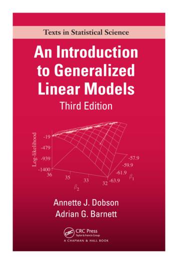
An Introductionto GeneralizedLinear ModelsThird EditionC9500 FM.indd 14/8/08 9:54:27 AM
CHAPMAN & HALL/CRCTexts in Statistical Science SeriesSeries EditorsBradley P. Carlin, University of Minnesota, USAJulian J. Faraway, University of Bath, UKMartin Tanner, Northwestern University, USAJim Zidek, University of British Columbia, CanadaAnalysis of Failure and Survival DataP. J. SmithThe Analysis of Time Series —An Introduction, Sixth EditionC. ChatfieldApplied Bayesian Forecasting and Time SeriesAnalysisA. Pole, M. West and J. HarrisonApplied Nonparametric Statistical Methods,Fourth EditionP. Sprent and N.C. SmeetonApplied Statistics — Handbook of GENSTATAnalysisE.J. Snell and H. SimpsonApplied Statistics — Principles and ExamplesD.R. Cox and E.J. SnellBayesian Data Analysis, Second EditionA. Gelman, J.B. Carlin, H.S. Sternand D.B. RubinBayesian Methods for Data Analysis,Third EditionB.P. Carlin and T.A. LouisBeyond ANOVA — Basics of AppliedStatisticsR.G. Miller, Jr.Computer-Aided Multivariate Analysis,Fourth EditionA.A. Afifi and V.A. ClarkA Course in Categorical Data AnalysisT. LeonardA Course in Large Sample TheoryT.S. FergusonData Driven Statistical MethodsP. SprentDecision Analysis — A Bayesian ApproachJ.Q. SmithElementary Applications of ProbabilityTheory, Second EditionH.C. TuckwellElements of SimulationB.J.T. MorganC9500 FM.indd 2Epidemiology — Study Design andData Analysis, Second EditionM. WoodwardEssential Statistics, Fourth EditionD.A.G. ReesExtending the Linear Model with R:Generalized Linear, Mixed Effects andNonparametric Regression ModelsJ.J. FarawayA First Course in Linear Model TheoryN. Ravishanker and D.K. DeyGeneralized Additive Models:An Introduction with RS. WoodInterpreting Data — A First Coursein StatisticsA.J.B. AndersonAn Introduction to GeneralizedLinear Models, Third EditionA.J. Dobson and A.G. BarnettIntroduction to Multivariate AnalysisC. Chatfield and A.J. CollinsIntroduction to Optimization Methods andTheir Applications in StatisticsB.S. EverittIntroduction to Probability with RK. BaclawskiIntroduction to Randomized ControlledClinical Trials, Second EditionJ.N.S. MatthewsIntroduction to Statistical Methods forClinical TrialsThomas D. Cook and David L. DeMetsLarge Sample Methods in StatisticsP.K. Sen and J. da Motta SingerLinear Models with RJ.J. FarawayMarkov Chain Monte Carlo —Stochastic Simulation for BayesianInference, Second EditionD. Gamerman and H.F. LopesMathematical StatisticsK. Knight4/8/08 9:54:27 AM
Modeling and Analysis of Stochastic SystemsV. KulkarniModelling Binary Data, Second EditionD. CollettModelling Survival Data in Medical Research,Second EditionD. CollettMultivariate Analysis of Variance and RepeatedMeasures — A Practical Approach forBehavioural ScientistsD.J. Hand and C.C. TaylorMultivariate Statistics — A Practical ApproachB. Flury and H. RiedwylPractical Data Analysis for DesignedExperimentsB.S. YandellPractical Longitudinal Data AnalysisD.J. Hand and M. CrowderPractical Statistics for Medical ResearchD.G. AltmanA Primer on Linear ModelsJ.F. MonahanProbability — Methods and MeasurementA. O’HaganProblem Solving — A Statistician’s Guide,Second EditionC. ChatfieldRandomization, Bootstrap andMonte Carlo Methods in Biology,Third EditionB.F.J. ManlyReadings in Decision AnalysisS. FrenchSampling Methodologies with ApplicationsP.S.R.S. RaoC9500 FM.indd 3Statistical Analysis of Reliability DataM.J. Crowder, A.C. Kimber,T.J. Sweeting, and R.L. SmithStatistical Methods for Spatial Data AnalysisO. Schabenberger and C.A. GotwayStatistical Methods for SPC and TQMD. BissellStatistical Methods in Agriculture andExperimental Biology, Second EditionR. Mead, R.N. Curnow, and A.M. HastedStatistical Process Control — Theoryand Practice, Third EditionG.B. Wetherill and D.W. BrownStatistical Theory, Fourth EditionB.W. LindgrenStatistics for AccountantsS. LetchfordStatistics for EpidemiologyN.P. JewellStatistics for Technology — A Course inApplied Statistics, Third EditionC. ChatfieldStatistics in Engineering —A Practical ApproachA.V. MetcalfeStatistics in Research and Development,Second EditionR. CaulcuttSurvival Analysis Using S —Analysis ofTime-to-Event DataM. Tableman and J.S. KimThe Theory of Linear ModelsB. JørgensenTime Series AnalysisH. Madsen4/8/08 9:54:27 AM
C9500 FM.indd 44/8/08 9:54:27 AM
Texts in Statistical ScienceAn Introductionto GeneralizedLinear ModelsThird EditionAnnette J. DobsonUniversity of QueenslandHerston, AustraliaAdrian G. BarnettQueensland University of TechnologyKelvin Grove, AustraliaC9500 FM.indd 54/8/08 9:54:28 AM
Chapman & Hall/CRCTaylor & Francis Group6000 Broken Sound Parkway NW, Suite 300Boca Raton, FL 33487-2742 2008 by Taylor & Francis Group, LLCChapman & Hall/CRC is an imprint of Taylor & Francis Group, an Informa businessNo claim to original U.S. Government worksPrinted in the United States of America on acid-free paper10 9 8 7 6 5 4 3 2 1International Standard Book Number-13: 978-1-58488-950-2 (Softcover)This book contains information obtained from authentic and highly regarded sources. Reasonableefforts have been made to publish reliable data and information, but the author and publisher cannot assume responsibility for the validity of all materials or the consequences of their use. Theauthors and publishers have attempted to trace the copyright holders of all material reproducedin this publication and apologize to copyright holders if permission to publish in this form has notbeen obtained. If any copyright material has not been acknowledged please write and let us know sowe may rectify in any future reprint.Except as permitted under U.S. Copyright Law, no part of this book may be reprinted, reproduced,transmitted, or utilized in any form by any electronic, mechanical, or other means, now known orhereafter invented, including photocopying, microfilming, and recording, or in any informationstorage or retrieval system, without written permission from the publishers.For permission to photocopy or use material electronically from this work, please access www.copyright.com (http://www.copyright.com/) or contact the Copyright Clearance Center, Inc. (CCC), 222Rosewood Drive, Danvers, MA 01923, 978-750-8400. CCC is a not-for-profit organization that provides licenses and registration for a variety of users. For organizations that have been granted aphotocopy license by the CCC, a separate system of payment has been arranged.Trademark Notice: Product or corporate names may be trademarks or registered trademarks, andare used only for identification and explanation without intent to infringe.Library of Congress Cataloging-in-Publication DataDobson, Annette J., 1945An introduction to generalized linear models / Annette J. Dobson and AdrianG. Barnett. -- 3rd ed.p. cm. -- (Chapman & Hall/CRC texts in statistical science series ; 77)Includes bibliographical references and index.ISBN 978-1-58488-950-2 (alk. paper)1. Linear models (Statistics) I. Barnett, Adrian G. II. Title. III. Series.QA276.D589 2008519.5--dc222008013034Visit the Taylor & Francis Web site athttp://www.taylorandfrancis.comand the CRC Press Web site athttp://www.crcpress.comC9500 FM.indd 64/8/08 9:54:28 AM
ContentsPreface1 Introduction1.1 Background1.2 Scope1.3 Notation1.4 Distributions related to the Normal distribution1.5 Quadratic forms1.6 Estimation1.7 Exercises111571112152 Model Fitting2.1 Introduction2.2 Examples2.3 Some principles of statistical modelling2.4 Notation and coding for explanatory variables2.5 Exercises1919193237403 Exponential Family and Generalized Linear Models3.1 Introduction3.2 Exponential family of distributions3.3 Properties of distributions in the exponential family3.4 Generalized linear models3.5 Examples3.6 Exercises454546485152554 Estimation4.1 Introduction4.2 Example: Failure times for pressure vessels4.3 Maximum likelihood estimation4.4 Poisson regression example4.5 Exercises5959596466695 Inference5.1 Introduction5.2 Sampling distribution for score statistics737374
5.35.45.55.65.75.8Taylor series approximationsSampling distribution for MLEsLog-likelihood ratio statisticSampling distribution for the devianceHypothesis testingExercises7677798085876 Normal Linear Models6.1 Introduction6.2 Basic results6.3 Multiple linear regression6.4 Analysis of variance6.5 Analysis of covariance6.6 General linear models6.7 Exercises898989951021141171187 Binary Variables and Logistic Regression7.1 Probability distributions7.2 Generalized linear models7.3 Dose response models7.4 General logistic regression model7.5 Goodness of fit statistics7.6 Residuals7.7 Other diagnostics7.8 Example: Senility and WAIS7.9 Exercises1231231241241311351381391401438 Nominal and Ordinal Logistic Regression8.1 Introduction8.2 Multinomial distribution8.3 Nominal logistic regression8.4 Ordinal logistic regression8.5 General comments8.6 Exercises1491491491511571621639 Poisson Regression and Log-Linear Models9.1 Introduction9.2 Poisson regression9.3 Examples of contingency tables9.4 Probability models for contingency tables9.5 Log-linear models9.6 Inference for log-linear models9.7 Numerical examples9.8 Remarks9.9 Exercises165165166171175177178179183183
10 Survival Analysis10.1 Introduction10.2 Survivor functions and hazard functions10.3 Empirical survivor function10.4 Estimation10.5 Inference10.6 Model checking10.7 Example: Remission times10.8 Exercises18718718919319519819920120211 Clustered and Longitudinal Data11.1 Introduction11.2 Example: Recovery from stroke11.3 Repeated measures models for Normal data11.4 Repeated measures models for non-Normal data11.5 Multilevel models11.6 Stroke example continued11.7 Comments11.8 Exercises20720720921321821922222422512 Bayesian Analysis12.1 Frequentist and Bayesian paradigms12.2 Priors12.3 Distributions and hierarchies in Bayesian analysis12.4 WinBUGS software for Bayesian analysis12.5 Exercises22922923323823824113 Markov Chain Monte Carlo Methods13.1 Why standard inference fails13.2 Monte Carlo integration13.3 Markov chains13.4 Bayesian inference13.5 Diagnostics of chain convergence13.6 Bayesian model fit: the DIC13.7 Exercises24324324324525525626026214 Example Bayesian Analyses14.1 Introduction14.2 Binary variables and logistic regression14.3 Nominal logistic regression14.4 Latent variable model14.5 Survival analysis14.6 Random effects14.7 Longitudinal data analysis14.8 Some practical tips for WinBUGS267267267271272275277279286
14.9 ex303
PrefaceThe original purpose of the book was to present a unified theoretical andconceptual framework for statistical modelling in a way that was accessible toundergraduate students and researchers in other fields.The second edition was expanded to include nominal and ordinal logisticregression, survival analysis and analysis of longitudinal and clustered data.It relied more on numerical methods, visualizing numerical optimization andgraphical methods for exploratory data analysis and checking model fit. Thesefeatures have been extended further in this new edition.The third edition contains three new chapters on Bayesian analysis. Thefundamentals of Bayesian theory were written long before the development ofclassical theory but practical Bayesian analysis has only recently become available. This availability is mostly thanks to Markov chain Monte Carlo methodswhich are introduced in Chapter 13. The increased availability of Bayesiananalysis means that more people with a classical knowledge of statistics aretrying Bayesian methods for generalized linear models. Bayesian analysis offerssignificant advantages over classical methods because of the ability formallyto incorporate prior information, greater flexibility and an ability to solvecomplex problems.This edition has also been updated with Stata and R code, which shouldhelp the practical application of generalized linear models. The chapters onBayesian analyses contain R and WinBUGS code.The data sets and outline solutions of the exercises are available on thepublisher’s website: http://www.crcpress.com/e products/downloads/.We are grateful to colleagues and students at the Universities of Queensland and Newcastle, Australia, and those taking postgraduate courses throughthe Biostatistics Collaboration of Australia for their helpful suggestions andcomments about the material.Annette Dobson and Adrian BarnettBrisbane
CHAPTER 1Introduction1.1 BackgroundThis book is designed to introduce the reader to generalized linear models;these provide a unifying framework for many commonly used statistical techniques. They also illustrate the ideas of statistical modelling.The reader is assumed to have some familiarity with classical statisticalprinciples and methods. In particular, understanding the concepts of estimation, sampling distributions and hypothesis testing is necessary. Experience inthe use of t-tests, analysis of variance, simple linear regression and chi-squaredtests of independence for two-dimensional contingency tables is assumed. Inaddition, some knowledge of matrix algebra and calculus is required.The reader will find it necessary to have access to statistical computingfacilities. Many statistical programs, languages or packages can now performthe analyses discussed in this book. Often, however, they do so with a differentprogram or procedure for each type of analysis so that the unifying structureis not apparent.Some programs or languages which have procedures consistent with theapproach used in this book are Stata, R, S-PLUS, SAS and Genstat. ForChapters 13 to 14 programs to conduct Markov chain Monte Carlo methodsare needed and WinBUGS has been used here. This list is not comprehensiveas appropriate modules are continually being added to other programs.In addition, anyone working through this book may find it helpful to be ableto use mathematical software that can perform matrix algebra, differentiationand iterative calculations.1.2 ScopeThe statistical methods considered in this book all involve the analysis of relationships between measurements made on groups of subjects or objects. Forexample, the measurements might be the heights or weights and the ages ofboys and girls, or the yield of plants under various growing conditions. Weuse the terms response, outcome or dependent variable for measurementsthat are free to vary in response to other variables called explanatory variables or predictor variables or independent variables—although thislast term can sometimes be misleading. Responses are regarded as randomvariables. Explanatory variables are usually treated as though they are non-
2INTRODUCTIONrandom measurements or observations; for example, they may be fixed by theexperimental design.Responses and explanatory variables are measured on one of the followingscales.1. Nominal classifications: e.g., red, green, blue; yes, no, do not know, notapplicable. In particular, for binary, dichotomous or binomial variablesthere are only two categories: male, female; dead, alive; smooth leaves,serrated leaves. If there are more than two categories the variable is calledpolychotomous, polytomous or multinomial.2. Ordinal classifications in which there is some natural order or ranking between the categories: e.g., young, middle aged, old; diastolic blood pressuresgrouped as 70, 71–90, 91–110, 111–130, 131 mmHg.3. Continuous measurements where observations may, at least in theory, fallanywhere on a continuum: e.g., weight, length or time. This scale includesboth interval scale and ratio scale measurements—the latter have a welldefined zero. A particular example of a continuous measurement is the timeuntil a specific event occurs, such as the failure of an electronic component;the length of time from a known starting point is called the failure time.Nominal and ordinal data are sometimes called categorical or discretevariables and the numbers of observations, counts or frequencies in eachcategory are usually recorded. For continuous data the individual measurements are recorded. The term quantitative is often used for a variable measured on a continuous scale and the term qualitative for nominal and sometimes for ordinal measurements. A qualitative, explanatory variable is calleda factor and its categories are called the levels for the factor. A quantitativeexplanatory variable is sometimes called a covariate.Methods of statistical analysis depend on the measurement scales of theresponse and explanatory variables.This book is mainly concerned with those statistical methods which arerelevant when there is just one response variable although there will usuallybe several explanatory variables. The responses measured on different subjectsare usually assumed to be statistically independent random variables althoughthis requirement is dropped in Chapter 11, which is about correlated data,and in subsequent chapters. Table 1.1 shows the main methods of statisticalanalysis for various combinations of response and explanatory variables andthe chapters in which these are described.The last three chapters are devotedto Bayesian methods which substantially extend these analyses.The present chapter summarizes some of the statistical theory used throughout the book. Chapters 2 through 5 cover the theoretical framework that iscommon to the subsequent chapters. Later chapters focus on methods foranalyzing particular kinds of data.Chapter 2 develops the main ideas of classical or frequentist statistical modelling. The modelling process involves four steps:
SCOPE3Table 1.1 Major methods of statistical analysis for response and explanatory variables measured on various scales and chapter references for this book. Extensions ofthese methods from a Bayesian perspective are illustrated in Chapters 12–14.Response (chapter)Explanatory variablesMethodsContinuous(Chapter 6)Binaryt-testNominal, 2 categoriesAnalysis of varianceOrdinalAnalysis of varianceContinuousMultiple regressionNominal & somecontinuousAnalysis ofcovarianceCategorical & continuousMultiple regressionCategoricalContingency tablesLogistic regressionContinuousLogistic, probit &other dose-responsemodelsCategorical & continuousLogistic regressionNominalContingency tablesCategorical & continuousNominal logisticregressionOrdinal(Chapter 8)Categorical & continuousOrdinal logisticregressionCounts(Chapter 9)CategoricalLog-linear modelsCategorical & continuousPoisson regressionFailure times(Chapter 10)Categorical & continuousSurvival analysis(parametric)Correlatedresponses(Chapter 11)Categorical & continuousGeneralizedestimating equationsMultilevel modelsBinary(Chapter 7)Nominal with 2 categories(Chapters 8 & 9)
4INTRODUCTION1. Specifying models in two parts: equations linking the response and explanatory variables, and the probability distribution of the response variable.2. Estimating fixed but unknown parameters used in the models.3. Checking how well the models fit the actual data.4. Making inferences; for example, calculating confidence intervals and testinghypotheses about the parameters.The next three chapters provide the theoretical background. Chapter 3 isabout the exponential family of distributions, which includes the Normal, Poisson and Binomial distributions. It also covers generalized linearmodels (as defined by Nelder and Wedderburn 1972). Linear regression andmany other models are special cases of generalized linear models. In Chapter 4methods of classical estimation and model fitting are described.Chapter 5 outlines frequentist methods of statistical inference for generalized linear models. Most of these methods are based on how well a modeldescribes the set of data. For example, hypothesis testing is carried out byfirst specifying alternative models (one corresponding to the null hypothesisand the other to a more general hypothesis). Then test statistics are calculatedwhich measure the “goodness of fit” of each model and these are compared.Typically the model corresponding to the null hypothesis is simpler, so if itfits the data about as well as a more complex model it is usually preferred onthe grounds of parsimony (i.e., we retain the null hypothesis).Chapter 6 is about multiple linear regression and analysis of variance (ANOVA). Regression is the standard method for relating a continuousresponse variable to several continuous explanatory (or predictor) variables.ANOVA is used for a continuous response variable and categorical or qualitative explanatory variables (factors). Analysis of covariance (ANCOVA) isused when at least one of the explanatory variables is continuous. Nowadaysit is common to use the same computational tools for all such situations. Theterms multiple regression or general linear model are used to cover therange of methods for analyzing one continuous response variable and multipleexplanatory variables.Chapter 7 is about methods for analyzing binary response data. The mostcommon one is logistic regression which is used to model relationships between the response variable and several explanatory variables which may becategorical or continuous. Methods for relating the response to a single continuous variable, the dose, are also considered; these include probit analysis which was originally developed for analyzing dose-response data frombioassays. Logistic regression has been generalized to include responses withmore than two nominal categories (nominal, multinomial, polytomous orpolychotomous logistic regression) or ordinal categories (ordinal logistic regression). These methods are discussed in Chapter 8.Chapter 9 concerns count data. The counts may be frequencies displayedin a contingency table or numbers of events, such as traffic accidents, whichneed to be analyzed in relation to some “exposure” variable such as the num-
NOTATION5ber of motor vehicles registered or the distances travelled by the drivers. Modelling methods are based on assuming that the distribution of counts can bedescribed by the Poisson distribution, at least approximately. These methodsinclude Poisson regression and log-linear models.Survival analysis is the usual term for methods of analyzing failure timedata. The parametric methods described in Chapter 10 fit into the frameworkof generalized linear models although the probability distribution assumed forthe failure times may not belong to the exponential family.Generalized linear models have been extended to situations where the responses are correlated rather than independent random variables. This mayoccur, for instance, if they are repeated measurements on the same subject or measurements on a group of related subjects obtained, for example,from clustered sampling. The method of generalized estimating equations (GEEs) has been developed for analyzing such data using techniquesanalogous to those for generalized linear models. This method is outlinedin Chapter 11 together with a different approach to correlated data, namelymultilevel modelling in which some parameters are treated as random variables rather than fixed but unknown constants. Multilevel modelling involvesboth fixed and random effects (mixed models) and relates more closely to theBayesian approach to statistical analysis.The main concepts and methods of Bayesian analysis are introduced inChapter 12. In this chapter the relationships between classical or frequentistmethods and Bayesian methods are outlined. In addition the software WinBUGS which is used to fit Bayesian models is introduced.Bayesian models are usually fitted using computer-intensive methods basedon Markov chains simulated using techniques based on random numbers.These methods are described in Chapter 13. This chapter uses some examplesfrom earlier chapters to illustrate the mechanics of Markov chain Monte Carlo(MCMC) calculations and to demonstrate how the results allow much richerstatistical inferences than are possible using classical methods.Chapter 14 comprises several examples, introduced in earlier chapters, whichare reworked using Bayesian analysis. These examples are used to illustrateboth conceptual issues and practical approaches to estimation, model fittingand model comparisons using WinBUGS.Further examples of generalized linear models are discussed in the books byMcCullagh and Nelder (1989), Aitkin et al. (2005) and Myers et al. (2001).Also there are many books about specific generalized linear models such asHosmer and Lemeshow (2000), Agresti (1990, 1996), Collett (2003a, 2003b),Diggle et al. (2002) and Goldstein (2003).1.3 NotationGenerally we follow the convention of denoting random variables by uppercase italic letters and observed values by the corresponding lower case letters.For example, the observations y1 , y2 , ., yn are regarded as realizations of the
6INTRODUCTIONrandom variables Y1 , Y2 , . . . , Yn . Greek letters are used to denote parametersand the corresponding lower case roman letters are used to denote estimatorsand estimates; occasionally the symbol b is used for estimators or estimates.For example, the parameter β is estimated by βb or b. Sometimes these conventions are not strictly adhered to, either to avoid excessive notation in caseswhere the meaning should be apparent from the context, or when there is astrong tradition of alternative notation (e.g., e or ε for random error terms).Vectors and matrices, whether random or not, are denoted by bold face lowerand upper case letters, respectively. Thus, y represents a vector of observations or a vector of random variables y1 . . yn Y1 . . ,Ynβ denotes a vector of parameters and X is a matrix. The superscript T isused for a matrix transpose or when a column vector is written as a row, e.g.,Ty [Y1 , . . . , Yn ] .The probability density function of a continuous random variable Y (or theprobability mass function if Y is discrete) is referred to simply as a probability distribution and denoted byf (y; θ)where θ represents the parameters of the distribution.We use dot (·) subscripts for summation and bars ( ) for means; thus,y N1 X1yi y·.N i 1NThe expected value and variance of a random variable Y are denoted byE(Y ) and var(Y ), respectively. Suppose random variables Y1 , . . . , YN are independent with E(Yi ) µi and var(Yi ) σi2 for i 1, . . . , n. Let the randomvariable W be a linear combination of the Yi ’sW a1 Y1 a2 Y2 . . . an Yn ,(1.1)where the ai ’s are constants. Then the expected value of W isE(W ) a1 µ1 a2 µ2 . . . an µn(1.2)var(W ) a21 σ12 a22 σ22 . . . a2n σn2 .(1.3)and its variance is
DISTRIBUTIONS RELATED TO THE NORMAL DISTRIBUTION71.4 Distributions related to the Normal distributionThe sampling distributions of many of the estimators and test statistics usedin this book depend on the Normal distribution. They do so either directly because they are derived from Normally distributed random variables or asymptotically, via the Central Limit Theorem for large samples. In this sectionwe give definitions and notation for these distributions and summarize therelationships between them. The exercises at the end of the chapter providepractice in using these results which are employed extensively in subsequentchapters.1.4.1 Normal distributions1. If the random variable Y has the Normal distribution with mean µ andvariance σ 2 , its probability density function is"11f (y; µ, σ ) exp 222πσ2 y µσ 2 #.We denote this by Y N(µ, σ 2 ).2. The Normal distribution with µ 0 and σ 2 1, Y N(0, 1), is called thestandard Normal distribution.3. Let Y1 , . . . , Yn denote Normally distributed random variables with Yi N(µi , σi2 ) for i 1, . . . , n and let the covariance of Yi and Yj be denoted bycov(Yi , Yj ) ρij σi σj ,where ρij is the correlation coefficient for Yi and Yj . Then the joint distribution of the Yi ’s is the multivariate Normal distribution with meanvector µ [µ1 , . . . , µn ]T and variance-covariance matrix V with diagonalelements σi2 and non-diagonal elements ρij σi σj for i 6 j. We write this asTy MVN(µ, V), where y [Y1 , . . . , Yn ] .4. Suppose the random variables Y1 , . . . , Yn are independent and Normallydistributed with the distributions Yi N(µi , σi2 ) for i 1, . . . , n. IfW a1 Y1 a2 Y2 . . . an Yn ,where the ai ’s are constants, then W is also Normally distributed, so that!nnnXXXW ai Yi Nai µi ,a2i σi2i 1i 1i 1by equations (1.2) and (1.3).1.4.2 Chi-squared distribution1. The central chi-squared distribution with n degrees of freedom is defined as the sum of squares of n independent random variables Z1 , . . . , Zn
8INTRODUCTIONeach with the standard Normal distribution. It is denoted byX2 nXi 1Zi2 χ2 (n).In matrix notation, if z [Z1 , . . . , Zn ]T , then zT z X 2 zTz χ2 (n).Pni 1Zi2 so that2. If X 2 has the distribution χ2 (n), then its expected value is E(X 2 ) n andits variance is var(X 2 ) 2n.3. If Y1 , . . . , Yn are independent, Normally distributed random variables, eachwith the distribution Yi N(µi , σi2 ), then 2n XYi µiX2 χ2 (n)(1.4)σii 1because each of the variables Zi (Yi µi ) /σi has the standard Normaldistribution N(0, 1).4. Let Z1 , . . . , Zn be independent random variables each with the distributionN(0, 1) and let Yi Zi µi , where at least one of the µi ’s is non-zero. Thenthe distribution ofXXXXX2Yi2 (Zi µi ) Zi2 2Zi µi µ2ihasmean n λ and larger variance 2n 4λ than χ2 (n) where λ P largerµ2i . This is called the non-central chi-squared distribution with ndegrees of freedom and non-centrality parameter λ. It is denoted byχ2 (n, λ).5. Suppose that the Yi ’s are not necessarily independent and the vector y T[Y1 , . . . , Yn ] has the multivariate Normal distribution y MVN(µ, V)where the variance–covariance matrix V is non-singular and its inverse isV 1 . ThenX 2 (y µ)T V 1 (y µ) χ2 (n).(1.5)6. More generally if y MVN(µ, V), then the random variable yT V 1 y hasthe non-central chi-squared distribution χ2 (n, λ) where λ µT V 1 µ.27. If X12 , . . . , Xmare m inde
Bayesian Data Analysis, Second Edition A. Gelman, J.B. Carlin, H.S. Stern and D.B. Rubin Bayesian Methods for Data Analysis, Third Edition B.P. Carlin and T.A. Louis Beyond ANOVA — Basics of Applied Statistics R.G. Miller, Jr. Computer-Aided Multivariate Analysis, Fourth Edition A.A. Afifi and V.A. Clark A Course in Categorical Data Analysis .
