Transcription
CHAPTER2MPLS TE Technology OverviewIn this chapter, you review the following topics: MPLS TE IntroductionBasic Operation of MPLS TEDiffServ-Aware Traffic EngineeringFast RerouteThis chapter presents a review of Multiprotocol Label Switching Traffic Engineering(MPLS TE) technology. MPLS TE can play an important role in the implementation ofnetwork services with quality of service (QoS) guarantees. The initial sections describe thebasic operation of the technology. This description includes the details of TE informationdistribution, path computation, and the signaling of TE LSPs. The subsequent sectionspresent how Differentiated Services (DiffServ)-Aware traffic engineering (DS-TE) helpsintegrate the implementation of DiffServ and MPLS TE. This chapter closes with a reviewof the fast reroute (FRR) capabilities in MPLS TE. Chapter 4, “Cisco MPLS TrafficEngineering,” covers in depth the Cisco implementation of MPLS TE in Cisco IOS andCisco IOS XR. In addition, Chapter 5, “Backbone Infrastructure,” discusses the differentnetwork designs that can combine QoS with MPLS TE.MPLS TE IntroductionMPLS networks can use native TE mechanisms to minimize network congestion andimprove network performance. TE modifies routing patterns to provide efficient mappingof traffic streams to network resources. This efficient mapping can reduce the occurrenceof congestion and improves service quality in terms of the latency, jitter, and loss thatpackets experience. Historically, IP networks relied on the optimization of underlyingnetwork infrastructure or Interior Gateway Protocol (IGP) tuning for TE. Instead, MPLSextends existing IP protocols and makes use of MPLS forwarding capabilities to providenative TE. In addition, MPLS TE can reduce the impact of network failures and increaseservice availability. RFC 2702 discusses the requirements for TE in MPLS networks.MPLS TE brings explicit routing capabilities to MPLS networks. An originating labelswitching route (LSR) (or headend) can set up a TE label switched path (LSP) to aterminating LSR (or tail end) through an explicitly defined path containing a list of
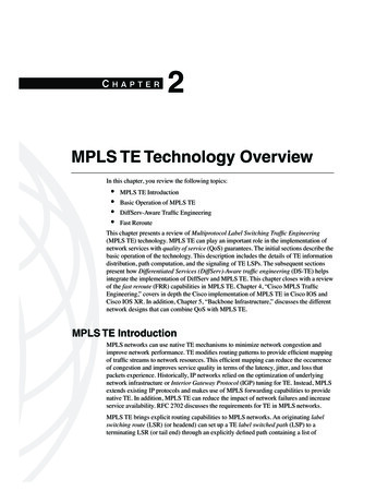
58Chapter 2: MPLS TE Technology Overviewintermediate LSRs (or midpoints). IP uses destination-based routing and does not providea general and scalable method for explicitly routing traffic. In contrast, MPLS networks cansupport destination-based and explicit routing simultaneously. MPLS TE uses extensionsto RSVP and the MPLS forwarding paradigm to provide explicit routing. Theseenhancements provide a level of routing control that makes MPLS suitable for TE.Figure 2-1 shows a sample MPLS network using TE. This network has multiple paths fromnodes A and E toward nodes D and H. In this figure, traffic from A and E toward D followsexplicitly routed LSPs through nodes B and C. Traffic from A and E toward H followsexplicitly routed LSPs through nodes F and G. Without TE, the IGP would compute theshortest path using only a single metric or cost. You could tune that metric, but that wouldprovide you limited capabilities to allocate network resources when compared with MPLSTE (specially, when you consider larger more complex network topologies). This chapterdescribes those routing and signaling enhancements that make MPLS TE possible.Figure 2-1Sample MPLS Network Using TEAEDIP/MPLSBCFGHMPLS TE also extends the MPLS routing capabilities with support for constraint-basedrouting. As mentioned earlier, IGPs typically compute routing information using a singlemetric. Instead of that simple approach, constraint-based routing can take into accountmore detailed information about network constraints, and policy resources. MPLS TEextends current link-state protocols (IS-IS and OSPF) to distribute such information.
Basic Operation of MPLS TE59Constraint-based routing and explicit routing allow an originating LSR to compute a paththat meets some requirements (constraints) to a terminating LSR and then set up a TE LSPthrough that path. Constraint-based routing is optional within MPLS TE. An offline tool canperform path computation and leave TE LSP signaling to the LSRs.MPLS TE supports preemption between TE LSPs of different priorities. Each TE LSP hasa setup and a holding priority, which can range from zero (best priority) through seven(worst priority). When a node signals a new TE LSP, other nodes throughout the pathcompare the setup priority of the new TE LSPs with the holding priority of existing TELSPs to make a preemption decision. A better setup priority can preempt worse-holdingpriorities a TE LSP can use hard or soft preemption. A node implementing hard preemptiontears down the existing TE LSP to accommodate the new TE LSP. In contrast, a nodeimplementing soft preemption signals back the pending preemption to the headend of theexisting TE LSP. The headend can then reroute the TE LSP without impacting the trafficflow. RFC 3209 and draft-ietf-mpls-soft-preemption-07. define TE LSP preemption.Basic Operation of MPLS TEThe operation of MPLS TE involves link information distribution, path computation, LSPsignaling, and traffic selection. This section explains the most important concepts behindeach of these four steps. LSRs implement the first two steps, link information distributionand path computation, when they need perform constraint-based routing. MPLS networksthat do not use constraint-based routing (or use an offline tool for that purpose) performonly LSP signaling and traffic selection. MPLS TE does not define any new protocols eventhough it represents a significant change in how MPLS networks can route traffic. Instead,it uses extensions to existing IP protocols.Link Information DistributionMPLS TE uses extensions to existing IP link-state routing protocols to distribute topologyinformation. An LSR requires detailed network information to perform constraint-basedrouting. It needs to know the current state of an extended list of link attributes to take a setof constraints into consideration during path computation for a TE LSP. Link-stateprotocols (IS-IS and OSPF) provide the flooding capabilities that are required to distributethese attributes. LSRs use this information to build a TE topology database. This databaseis separate from the regular topology database that LSRs build for hop-by-hop destinationbased routing.MPLS TE introduces available bandwidth, an administrative group (flags), and a TE metricas new link attributes. Each link has eight amounts of available bandwidth correspondingto the eight priority levels that TE LSPs can have. The administrative group (flags) acts as
60Chapter 2: MPLS TE Technology Overviewa classification mechanism to define link inclusion and exclusion rules. The TE metric is asecond link metric for path optimization (similar to the IGP link metric). In addition, LSRsdistribute a TE ID that has a similar function to a router ID. The OSPF and IS-IS extensionsmirror each other and have the same semantics. Table 2-1 shows the complete list of linkattributes. RFC 3784 and RFC 3630 define the IS-IS and OSPF extensions for TErespectively.Table 2-1NOTEExtended Link Attributes Distributed for TELink AttributeDescriptionInterface addressIP address of the interface corresponding to the linkNeighbor addressIP address of the neighbor’s interface corresponding to the linkMaximum link bandwidthTrue link capacity (in the neighbor direction)Reservable link bandwidthMaximum bandwidth that can be reserved (in the neighbordirection)Unreserved bandwidthAvailable bandwidth at each of the (eight) preemption priority levels(in the neighbor direction)TE metricLink metric for TE (may differ from the IGP metric)Administrative groupAdministratively value (flags) associated with the link for inclusion/exclusion policiesIn addition to the attributes listed in Table 2-1, OSPF advertises the link type (point-to-pointor multi-access) and a link ID. OSPF uses type 10 opaque (area-local scope) link-stateadvertisements (LSA) to distribute this information.MPLS TE can still perform constraint-based routing in the presence of multiple IGP areasor multiple autonomous systems. OSPF and IS-IS use the concept of areas or levels to limitthe scope of information flooding. An LSR in a network with multiple areas only builds apartial topology database. The existence of these partial databases has some implicationsfor path computation, as the next section describes. LSRs in an inter-autonomous systemTE environment also need to deal with partial network topologies. Fortunately, inter-areaTE and inter-autonomous system TE use similar approaches for constraint-based routing inthe presence of partial topology information.Path ComputationLSRs can perform path computation for a TE LSP using the TE topology database. Acommon approach for performing constraint-based routing on the LSRs is to use anextension of the shortest path first (SPF) algorithm. This extension to the original algorithm
Basic Operation of MPLS TE61generally receives the name of constraint-based, shortest path first (CSPF). The modifiedalgorithm executes the SPF algorithm on the topology that results from the removal of thelinks that do not meet the TE LSP constraints. The algorithm may use the IGP link metricor the link TE metric to determine the shortest path. CSPF does not guarantee a completelyoptimal mapping of traffic streams to network resources, but it is considered an adequateapproximation. MPLS TE specifications do not require that LSRs perform pathcomputation or attempt to standardize a path computation algorithm.Figure 2-2 illustrates a simplified version of CSPF on a sample network. In this case,node E wants to compute the shortest path to node H with the following constraints: onlylinks with at least 50 bandwidth units available and an administrative group value of 0xFF.Node E examines the TE topology database and disregards links with insufficientbandwidth or administrative group values other than 0xFF. The dotted lines in the topologyrepresent links that CSPF disregards. Subsequently, node E executes the shortest pathalgorithm on the reduced topology using the link metric values. In this case, the shortestpath is {E, F, B, C, H}. Using this result, node E can initiate the TE LSP signaling.Figure 2-2Path Computation Using the CSPF AlgorithmETE Topology DatabaseABW 50Metric 20Admin grp 0xFFBW 100Metric 20Admin grp 0x00BW 200Metric 10Admin grp 0xFFBBW 100Metric 10Admin grp 0xFFBW 40Metric 20Admin grp 0xFFCDBW 60Metric 20Admin grp 0xFFBW 80Metric 10Admin grp 0xFFBW 50Metric 20Admin grp 0xFFFEBW 30Metric 20Admin grp 0xFFBW 100Metric 20Admin grp 0xFFLink does not meet constraints.Link meets constraints.BW 200Metric 10Admin grp 0x00GBW 100Metric 20Admin grp 0xFFH
62Chapter 2: MPLS TE Technology OverviewPath computation in multi-area or inter-autonomous system environments may involveseveral partial computations along the TE LSP. When the headend does not have a completeview of the network topology, it can specify the path as a list of predefined boundary LSR(Area Border Router [ABR] in the case of inter-area and Autonomous System BoundaryRouter [ASBR] in the case of inter-autonomous system). The headend can compute a path tothe first boundary LSR (which must be in its topology database and initiate the signalling ofthe TE LSP signaling can be initiated). When the signaling reaches the boundary LSR, thatLSR performs the path computation to the final destination if it is in its topology. If thedestination is not in the topology, the signaling should indicate the next exit boundary LSR,and the path computation will take place to that boundary LSR. The process continues untilthe signaling reaches the destination. This process of completing path computation during TELSP signaling is called loose routing.Figure 2-3 shows path computation in a sample network with multiple IGP areas. All LSRs havea partial network topology. The network computes a path between nodes E and H crossing thethree IGP areas in the network. Node E selected nodes F and G, which have as the boundaryLSRs that the TE LSP will traverse. Node E computes the path to node F and initiates the TELSP signaling. When node F receives the signaling message, it computes the next segment ofthe path toward node G. When the signaling arrives at node G, it completes the path computationtoward node H in area 2. The next section explains how LSRs signal TE LSPs.Figure 2-3Multi-Area Path ComputationIP/MPLSADBICFJGEHArea 1Area 0Area 2AEDBBICCFFJGGH
Basic Operation of MPLS TE63Signaling of TE LSPsMPLS TE introduces extensions to RSVP to signal up LSPs. RSVP uses five new objects:LABEL REQUEST, LABEL, EXPLICIT ROUTE, RECORD ROUTE, andSESSION ATTRIBUTE. RSVP Path messages use a LABEL REQUEST object torequest a label binding at each hop. Resv messages use a LABEL object to perform labeldistribution. Network nodes perform downstream-on-demand label distribution using thesetwo objects. The EXPLICIT ROUTE object contains a hop list that defines the explicitrouted path that the signaling will follow. The RECORD ROUTE object collects hop andlabel information along the signaling path. The SESSION ATTRIBUTE object lists theattribute requirements of the LSP (priority, protection, and so forth).RFC 3209 defines these RSVP TE extensions. Table 2-2 summarizes the new RSVP objectsand their function.NOTEThe Internet Engineering Task Force (IETF) considered extensions to the LabelDistribution Protocol (LDP) as a signaling protocol for TE LSPs in the early stages ofMPLS TE. These protocol extensions were called Constraint-based routed LDP (CRLDP). For some time, CR-LDP and RSVP TE specifications advanced simultaneously. In2002, the MPLS working group at the IETF decided not to pursue new developments forCR-LDP and focused instead on RSVP TE as the prime protocol for MPLS TE.Table 2-2New RSVP Objects to Support MPLS TERSVP ObjectRSVP MessageDescriptionLABEL REQUESTPathLabel request to downstream neighborLABELResvMPLS label allocated by downstream neighborEXPLICIT ROUTEPathHop list defining the course of the TE LSPRECORD ROUTEPath, ResvHop/label list recorded during TE LSP setupSESSION ATTRIBUTEPathRequested LSP attributes (priority, protection,affinities)Figure 2-4 illustrates the setup of a TE LSP using RSVP. In this scenario, node E signals aTE LSP toward node H. RSVP Path messages flow downstream with a collection of objects,four of which are related to MPLS TE (EXPLICIT ROUTE, LABEL REQUEST,SESSION ATTRIBUTE, and RECORD ROUTE). Resv messages flow upstream andinclude two objects related to MPLS TE (LABEL and RECORD ROUTE). Each nodeperforms admission control and builds the LSP forwarding information base (LFIB) whenprocessing the Resv messages. The structure of the LFIB and the MPLS forwarding
64Chapter 2: MPLS TE Technology Overviewalgorithm remain the same regardless of the protocols that populated the information (forexample, RSVP in the case of MPLS TE).Figure 2-4TE LSP Setup Using RSVPRSVP MessagesStructureRSVP Message Forwarding BetweenHead End and Tail EndPath MessageSESSIONARSVP HOPDIP/MPLSTIME VALUESEXPLICIT ROUTEBCLABEL REQUESTSESSION ATTRIBUTESENDER TEMPLATESENDER TSPEC21ADSPEC12PathRECORD ROUTEPath14ResvLabel 20Resv Message2SESSION3FResv 4Label 35Path3GResvLabel 3HERSVP HOPTIME VALUESSTYLENode E LFIBFLOWSPECFILTER SPECInputLabelNode F LFIBOutput OutputInterface LabelInputLabelNode G LFIBOutput OutputInterface LabelInputLabelNode H LFIBOutput OutputInterface LabelInputLabelOutput OutputInterface LabelLABELRECORD ROUTE—2202033535333——Traffic SelectionMPLS TE separates TE LSP creation from the process of selecting the traffic that will usethe TE LSP. A headend can signal a TE LSP, but traffic will start flowing through the LSPafter the LSR implements a traffic-selection mechanism. Traffic can enter the TE LSP onlyat the headend. Therefore, the selection of the traffic is a local head-end decision that canuse different approaches without the need for standardization. The selection criteria can bestatic or dynamic. It can also depend on the packet type (for instance, IP or Ethernet) orpacket contents (for example, class of service). An MPLS network can make use of severaltraffic-selection mechanisms depending on the services it offers.DiffServ-Aware Traffic EngineeringMPLS DS-TE enables per-class TE across an MPLS network. DS-TE provides moregranular control to minimize network congestion and improve network performance.DS-TE retains the same overall operation framework of MPLS TE (link information
DiffServ-Aware Traffic Engineering65distribution, path computation, signaling, and traffic selection). However, it introducesextensions to support the concept of multiple classes and to make per-class constraint-basedrouting possible. These routing enhancements help control the proportion of traffic ofdifferent classes on network links. RFC 4124 introduces DS-TE protocol extensions.Both DS-TE and DiffServ control the per-class bandwidth allocation on network links. DSTE acts as a control-plane mechanism, while DiffServ acts in the forwarding plane. Ingeneral, the configuration in both planes will have a close relationship. However, they donot have to be identical. They can use a different number of classes and different relativebandwidth allocations to satisfy the requirements of particular network designs. Figure 2-5shows an example of bandwidth allocation in DiffServ and DS-TE for a particular link. Inthis case, the link rate equals the maximum reservable bandwidth for TE. Each classreceives a fraction of the total bandwidth amount in the control and forwarding planes.However, the bandwidth proportions between classes differ slightly in this case.DS-TE does not imply the use of Label-inferred-class LSP (L-LSPs). An MPLS node maysignal a DS-TE LSP as an EXP-inferred-class LSP (E-LSP) or L-LSP. Furthermore, a DSTE LSP may not signal any DiffServ information or not even count on the deployment ofDiffServ on the network. You need to keep in mind that an instance of a class within DSTE does not need to maintain a one-to-one relationship with a DiffServ class. Chapter 5explains different models of interaction between TE and DiffServ.Figure 2-5Bandwidth Allocation in DiffServ and DS-TEForwarding PlaneControl BandwidthDiffServBandwidthAllocationLink RateThis section uses the term aggregate MPLS TE to refer to MPLS TE without the DS-TEextensions. Even though that name might not be completely accurate in some MPLS TEdesigns, it differentiates TE with a single bandwidth constraint from the approach thatDS-TE uses.
66Chapter 2: MPLS TE Technology OverviewClass-Types and TE-ClassesDS-TE uses the concept of Class-Type (CT) for the purposes of link bandwidth allocation,constraint-based routing, and admission control. A network can use up to eight CTs (CT0through CT7). DS-TE retains support for TE LSP preemption, which can operate within aCT or across CTs. TE LSPs can have different preemption priorities regardless of their CT.CTs represent the concept of a class for DS-TE in a similar way that per-hop behavior(PHB) scheduling class (PSC) represents it for DiffServ. Note that flexible mappingsbetween CTs and PSCs are possible. You can define a one-to-one mapping between CTsand PSCs. Alternatively, a CT can map to several PSCs, or several CTs can map to one PSC.DS-TE provides flexible definition of preemption priorities while retaining the samemechanism for distribution of unreserved bandwidth on network links. DS-TE redefines themeaning of the unreserved bandwidth attribute discussed in the section “Link InformationDistribution” without modifying its format. When DS-TE is in use, this attribute representsthe unreserved bandwidth for eight TE classes. A TE-Class defines a combination of a CTand a corresponding preemption priority value. A network can use any 8 (TE-Class)combinations to use out of 64 possible combinations (8 CTs times 8 priorities). No relativeordering exists between the TE-Classes, and a network can use a subset of the 8 possiblevalues. However, the TE-Class definitions must be consistent across the DS-TE network.Tables 2-3, 2-4, and 2-5 include examples of three different TE-Class definitions: Table 2-3Table 2-3 illustrates a TE-Class definition that is backward compatible with aggregateMPLS TE. In this example, all TE-Classes support only CT0, with 8 differentpreemption priorities ranging from 0 through 7.Table 2-4 presents a second example where the TE-Class definition uses 4 CTs (CT0,CT1, CT2, and CT3), with 8 preemption priority levels (0 and 7) for each CT. Thisdefinition makes preemption possible within CTs but not across CTs.Table 2-5 contains a TE-Class definition with 2 CTs (CT0 and CT1) and 2 preemptionpriority levels (0 and 7). 2 third example defines some TE-Classes as unused. In thiscase, preemption is possible within and across CTs. With this design, preemption ispossible within and across CTs, but you can signal CT1 TE LSPs (using priority zero)that no other TE LSP can preempt.TE-Class Definition Backward Compatible with Aggregate MPLS TETE-ClassCTPriority000101202303404505606707
DiffServ-Aware Traffic EngineeringTable 2-4Table 2-5Table 2-6TE-Class Definition with Four CTs and 8 Preemption PrioritiesTE ClassClass TypePriority007106215314423522631730TE-Class Definition with Two CTs and Two Preemption usedUnused4005106UnusedUnused7UnusedUnusedTE-Class Definition with Two CTs and Eight Preemption 1067
68Chapter 2: MPLS TE Technology OverviewDS-TE introduces a new CLASSTYPE RSVP object. This object specifies the CTassociated with the TE LSP and can take a value ranging form one to seven. DS-TE nodesmust support this new object and include it in Path messages, with the exception of CT0 TELSPs. The Path messages associated with those LSPs must not use the CLASSTYPE objectto allow non-DS-TE nodes to interoperate with DS-TE nodes. Table 2-6 summarizes theCLASSTYPE object.Table 2-7New RSVP Object for DS-TERSVP ObjectRSVP MessageFRR FunctionCLASSTYPEPathCT associated with the TE LSP. Not used for CT0 forbackward compatibility with non-DS-TE nodes.Bandwidth ConstraintsA set of bandwidth constraints (BC) defines the rules that a node uses to allocate bandwidthto different CTs. Each link in the DS-TE network has a set of BCs that applies to the CTsin use. This set may contain up to eight BCs. When a node using DS-TE admits a new TELSP on a link, that node uses the BC rules to update the amount of unreserved bandwidthfor each TE-Class. One or more BCs may apply to a CT depending on the model.DS-TE can support different BC models. The IETF has primarily defined two BC models:maximum allocation model (MAM) and Russian dolls model (RDM). These are discussedin the following subsections of this chapter.DS-TE also defines a BC extension for IGP link advertisements. This extension complementsthe link attributes that Table 2-1 already described and applies equally to OSPF and IS-IS.Network nodes do not need this BC information to perform path computation. They rely onthe unreserved bandwidth information for that purpose. However, they can optionally useit to verify DS-TE configuration consistency throughout the network or as a path computationheuristic (for instance, as a tie breaker for CSPF). A DS-TE deployment could use differentBC models throughout the network. However, the simultaneous use of different modelsincreases operational complexity and can adversely impact bandwidth optimization. Table2-8 summarizes the BC link attribute that DS-TE uses.Table 2-8Optional BC Link Attribute Distributed for DS-TELink AttributeDescriptionBCsBC model ID and BCs (BC0 through BCn) that the link uses for DS-TEMaximum Allocation ModelThe MAM defines a one-to-one relationship between BCs and Class-Types. BCn definesthe maximum amount of reservable bandwidth for CTn, as Table 2-9 shows. The use ofpreemption does not affect the amount of bandwidth that a CT receives. MAM offers
DiffServ-Aware Traffic Engineering69limited bandwidth sharing between CTs. A CT cannot make use of the bandwidth leftunused by another CT. The packet schedulers managing congestion in the forwarding planetypically guarantee bandwidth sharing. To improve bandwidth sharing using MAM, youmay make the sum of all BCs greater than the maximum reservable bandwidth. However,the total reserved bandwidth for all CTs cannot exceed the maximum reservable bandwidthat any time. RFC 4125 defines MAM.Table 2-9MAM Bandwidth Constraints for Eight CTsBandwidth ConstraintMaximum Bandwidth Allocation 0Figure 2-6 shows an example of a set of BCs using MAM. This DS-TE configuration usesthree CTs with their corresponding BCs. In this case, BC0 limits CT0 bandwidth to15 percent of the maximum reservable bandwidth. BC1 limits CT1 to 50 percent, and BC2limits CT2 to 10 percent. The sum of BCs on this link is less than its maximum reservablebandwidth. Each CT will always receive its bandwidth share without the need for preemption.Preemption will not have an effect on the bandwidth that a CT can use. This predictabilitycomes at the cost of no bandwidth sharing between CTs. The lack of bandwidth sharing canforce some TE LSPs to follow longer paths than necessary.Figure 2-6MAM Constraint Model ExampleBC0 15%CT0CT1BC1 50%BC2 10%CT2MaximumReservableBandwidth
70Chapter 2: MPLS TE Technology OverviewRussian Dolls ModelThe RDM defines a cumulative set of constraints that group CTs. For an implementationwith n CTs, BCn always defines the maximum bandwidth allocation for CTn. Subsequentlower BCs define the total bandwidth allocation for the CTs at equal or higher levels. BC0always defines the maximum bandwidth allocation across all CTs and is equal to themaximum reservable bandwidth of the link.Table 2-10 shows the RDM BCs for a DS-TE implementation with eight CTs. The recursivedefinition of BCs improves bandwidth sharing between CTs. A particular CT can benefitfrom bandwidth left unused by higher CTs. A DS-TE network using RDM can rely on TELSP preemption to guarantee that each CT gets a fair share of the bandwidth. RFC 4127defines RDM.Table 2-10RDM Bandwidth Constrains for Eight CTsBandwidth ConstraintMaximum Bandwidth Allocation ForBC7CT7BC6CT7 CT6BC5CT7 CT6 CT5BC4CT7 CT6 CT5 CT4BC3CT7 CT6 CT5 CT4 CT3BC2CT7 CT6 CT5 CT4 CT3 CT2BC1CT7 CT6 CT5 CT4 CT3 CT2 CT1BC0 Maximum reservablebandwidthCT7 CT6 CT5 CT4 CT3 CT2 CT1 CT0Figure 2-7 shows an example of a set of BCs using RDM. This DS-TE implementation usesthree CTs with their corresponding BCs. In this case, BC2 limits CT2 to 30 percent of themaximum reservable bandwidth. BC1 limits CT2 CT1 to 70 percent. BC0 limitsCT2 CT1 CT0 to 100 percent of the maximum reservable bandwidth, as is always the casewith RDM. CT0 can use up to 100 percent of the bandwidth in the absence of CT2 and CT1TE LSPs. Similarly, CT1 can use up to 70 percent of the bandwidth in the absence of TELSPs of the other two CTs. CT2 will always be limited to 30 percent when no CT0 or CT1TE LSPs exist. The maximum bandwidth that a CT receives on a particular link depends onthe previously signaled TE LSPs, their CTs, and the preemption priorities of all TE LSPs.Table 2-11 compares MAM and RDM.
Fast RerouteFigure 2-7RDM Constraint Model ExampleBC0 MRBCT1 CT2BC1 70%BC2 30%Table 2-1171CT0 CT1 CT2MaximumReservableBandwidth(MRB)CT2Comparing MAM and RDM BC ModelsMAMRDM1 BC per CT.1 or more CTs per BC.Sum of all BCs may exceed maximum reservablebandwidth.BC0 always equals the maximum reservablebandwidth.Preemption not required to provide bandwidthguarantees per CT.Preemption required to provide bandwidthguarantees per CT.Bandwidth efficiency and protection against QoSdegradation are mutually exclusive.Provides bandwidth efficiency and protectionagainst QoS degradation simultaneously.Fast RerouteMPLS TE supports local repair of TE LSPs using FRR. Traffic protection in case of anetwork failure is critical for real-time traffic or any other traffic with strict packet-lossrequirements. In particular, FRR uses a local protection approach that relies on apresignaled backup TE LSP to reroute traffic in case of a failure. The node immediatelynext to the failure is responsible for rerouting the traffic and is the headend of the backupTE LSP. Therefore, no delay occurs in the propagation of the failure condition, and no delayoccurs in computing a path and signaling a new TE LSP to reroute the traffic. FRR canreroute traffic in tens of milliseconds. RFC 4090 describes the operation and the signalingextensions that MPLS TE FRR requires.
72Chapter 2: MPLS TE Technology OverviewNOTEMPLS TE FRR specifications offer two protection techniques: facility backup and one-toone backup. Facility backup uses label stacking to reroute multiple protected TE LSPsusing a single backup TE LSP. One-to-one backup does not use label stacking, and everyprotected TE LSP requires a dedicated backup TE LSP. The remainder of this sectionfocuses on the facility backup approach because of its greater scalability and wider use.Figure 2-8 shows an example of an MPLS network using FRR. In this case, node E signalsa TE LSP toward node H. The network protects this TE LSP against a failure of the linkbetween nodes F and G. Given the local protection nature of FRR, node F is responsible forrerouting the traffic into the backup TE LSP in case the link between nodes F and G fails.This role makes node F the point of local repair (PLR). It has presignaled a backup TE LSPthrough node I toward node G to bypass the potential link failure. The PLR is always theheadend of the backup TE LSP. Node G receives the name of merge point (MP) and is thenode where the protected traffic will exit the backup TE LSP during the failure and retakethe original path of the protected TE LSP.Figure 2-8MPLS Network Using FRRIP/MPLSABDCIEFPoint o
This chapter presents a review of Multiprotocol Label Switching Traffic Engineering (MPLS TE) technology. MPLS TE can play an important role in the implementation of . view of the network topology, it can specify the path as a list of predefined boundary LSR (Area Border Router [ABR] in the case of inter-area and Autonomous System Boundary