Transcription
23rd International Congress on Modelling and Simulation, Canberra, ACT, Australia, 1 to 6 December 2019mssanz.org.au/modsim2019Estimating bankfull channel geometry, dimensions andassociated hydraulic attributes using high resolutionDEM generated from LiDAR dataB. FentieDepartment of Environment and Science, Queensland, AustraliaEmail: banti.fentie@des.qld.gov.auAbstract: Knowledge on river channel dimensions at bankfull flow is essential for flood forecasting, streamrehabilitation and bank stabilization works, environmental flow modelling, and streambank erosion modelling.The difficulty of collecting spatially distributed, high-resolution data on channel form and behaviour made itnecessary for broad scale erosion models to adopt generalised approaches to bankfull flow estimation. Thesetechniques are commonly based on simple hydraulic formulae applied to cross-sectional averages. It isrecognized that these generalised estimations frequently fail to describe the non-uniform flow and transportconditions observed in natural rivers. Application of Dynamic SedNet in the catchment water quality modellingproject of Paddock to Reef Integrated Monitoring, Modelling and Reporting Program (P2R) under Reef Planuses relationships between channel width and height with contributing catchment area that are regionallygenerated to determine these river channel dimensions. There are obvious shortcomings of this approachincluding: (1) the fact that channel dimensions are greatly spatially variable even when values of theexplanatory variable are the same (e.g., bankfull flow occurs more often on coastal plains), (2) limited datapoints used to generate the empirical equation. However, with recent advances in the area of generating highresolution digital elevation models (DEMs) from Light Detection And Ranging (LiDAR) data and availabilityof tools to process them, it may be possible to determine channel geometry and dimensions in a more robustand reliable way. Conventional topographic LiDAR, such as that used to generate theDEM used in this study, does not penetrate water bodies. In these situations, waterpenetrating LiDAR (Bathymetric LiDAR) will need to be employed. However, in lowflow situations, as in the current study, and/or where flow depth can be determined frommonitoring, it is possible to subtract flow depth from the water surface elevation toestimate channel-bed elevation and height.This study demonstrates how a high resolution DEM generated from LiDAR data inconjunction with estimates of flow depth, which was low at the time of LiDAR dataacquisition, can be used to generate bankfull river channel width and height therebyallowing estimation of other river flow parameters. Figure 1 shows the workflow (stepsfollowed) in order to achieve this.Bankfull flow parameter values estimated from the approach currently employed in P2Rand those estimated in this study (e.g. flow cross-sectional area, wetted perimeter, andhydraulic radius) have been compared at two modelled stream reaches where LiDARDEM is available. The comparison shows that the P2R approach overestimates allbankfull flow attributes. However, since Dynamic SedNet uses a user-specifiedrecurrence interval to determine bankfull discharge and applies a calibration coefficientfor adjusting bank erosion, the model may not necessarily overestimate streambankerosion. Nevertheless, the reliance on a calibration coefficient to account for input datalimitations reduces confidence in model predictions, as it could lead to situations Figure 1. Workflow forwhere the model gives the right answer for the wrong reason which will inhibit estimating river channeldimensions fromparameter transfer outside the calibration dataset.LiDAR DEMThis paper has: (1) demonstrated that the approach adopted in this study using LiDARDEM may be a more reliable alternative than determining river channel dimensions as a power function ofcatchment area, and the application of the concept of recurrence interval in estimating bankfull flow, and (2)shown that the assumption of rectangular river channel geometry in the application of Dynamic SedNet in P2Ris overestimating bankfull flow and associated hydraulic attributes such as hydraulic radius in the case studyreaches.Keywords:Channel dimensions, Dynamic SedNet, hydraulic parameters, Mary Catchment1098
B. Fentie, Estimating bankfull channel geometry, dimensions and associated hydraulic attributes using highresolution DEM generated from LiDAR data1.INTRODUCTIONKnowledge on river channel dimensions at bankfull flow is essential for flood forecasting, stream rehabilitationand bank stabilisation works, environmental flow modelling, and streambank erosion modelling. The difficultyof collecting spatially distributed, high-resolution data on channel form and behaviour made it necessary forbroad scale erosion models to adopt generalised approaches to bankfull flow estimation. These techniques arecommonly based on simple hydraulic formulae applied to cross-sectional averages. It is recognized that thesegeneralised estimations frequently fail to describe the non-uniform flow and transport conditions observed innatural rivers. Application of Dynamic SedNet in the Paddock to Reef (P2R) catchment water qualitymodelling project of the Reef Plan uses relationships between channel width and height with contributingcatchment area that are regionally generated to determine these river channel dimensions. To alleviate thisproblem, power-law relationships that are unique to the hydrometeorology of the catchment have been used toestimate River channel width (W) and channel height (H) as a function of mean annual discharge (Q). Theserelationships can also be expressed with respect to contributing area (A) instead of discharge (Q) (Fisher et al.,2013). The plots of the regression equations for bankfull channel dimensions and drainage area are commonlyreferred to as regional curves. Regional curves are based on simple regression equations, which use oneexplanatory variable (e.g., drainage area) to estimate the response variables of bankfull width, bankfull depth,bankfull cross-sectional area, and bankfull discharge.The estimation of stream channel attributes for the Dynamic SedNet model (Wilkinson et al., 2013, Ellis andSearle, 2014), a plug-in for the Source modelling framework, for the modelling component of P2R is anexample of methods that use power-law relationships between channel width and height with contributingcatchment area. However, there are shortcomings of estimating these stream channel attributes as a function ofjust catchment area including: (1) the fact that channel dimensions and hence bankfull flow are spatiallyvariable even when values of the explanatory variable are the same (e.g., bankfull flow occurs more often oncoastal plains), and (2) limited data points used to generate the empirical equation. Nevertheless, with recentadvances in generation of high resolution digital elevation models (DEM) from Light Detection And Ranging(LiDAR) data and availability of tools to process them (e.g., River Bathymetry Toolkit (McKean et al., 2009),Hec-GeoRAS (US Army Corp of Engineers), FluvialCorridor (Roux, et al., 2015)), it is possible to determinethese channel dimensions in a more robust and reliable way. Furthermore, where there is a time-series ofLiDAR data, it is possible to estimate soil erosion from elevation differences between resulting chronosequential DEMs (i.e., DEM of Difference). However, conventional LiDAR does not penetrate water bodiesand additional bathymetric measurements are necessary to complete any parts of a DEM which were underwater at the time of the LiDAR acquisition (Smart et al., 2009). On the other hand, for reaches with fairlyconstant and shallow flow of less than 2 m (which was the case in this study), it may be possible to adopt aconstant, representative depth. The average flow depth is then subtracted from the corresponding water surfaceelevation to give the local bed elevation and thereby the channel height. The bankfull height in this study isthen determined visually from the cross-sectional profile of the channel.With the aim of providing a relative study on the potential use of different DEMs to estimate useful hydraulicinformation, such as water stage, Schumann et al. (2008) compared water stages derived from LiDAR,topographic contours and SRTM Shuttle Radar Topography mission (SRTM). They found that results fromLiDAR were by far the most accurate, despite the fact that, for the flood-prone area in their study, the othertwo sources of DEMs also performed reasonably well.One assumption made in Dynamic SedNet is that river channels are of rectangular geometry. However, mostnatural and man-made channels are irregular or trapezoidal in cross-section. Unlike models such as SWAT andHSPF/LSPC (Bicknell et al., 2001), which assume trapezoidal river channel cross-section, Dynamic SedNetadopts a rectangular channel cross-section to model stream bank erosion. This study will demonstratedifferences in the magnitudes of different channel attributes with and without this assumption.The objectives of this paper were twofold:1. demonstrate that, where it is available, application of LiDAR DEM may be a more reliable alternativethan the current approach adopted by P2R when informing Dynamic SedNet of river channeldimensions and bankfull flow estimation, and1099
B. Fentie, Estimating bankfull channel geometry, dimensions and associated hydraulic attributes using highresolution DEM generated from LiDAR data2.show that the assumption of rectangular river channelgeometry in Dynamic SedNet overestimates bankfull flowand associated hydraulic attributes such as hydraulic radius inthe case study reaches.2.METHODS2.1.The study areaCovering a total area of some 9,420 km², the Mary River catchment (seelocation in Figure 2) has a sub-humid and subtropical climate. Averageannual rainfall varies from about 2,000 mm/yr in the far southeast, toabout 800 mm/yr in the west. This study was undertaken on a 26-kmsection of the middle reaches of Mary River, between its confluenceswith Wide Bay Creek and Munna Creek. The adopted middle threaddistances (AMTDs) for these stream junctions are 136 km and 110 kmrespectively. The subject section of the river is highlighted in red in theleft map and expanded on the right map (Figure 3).The Miva gauging station (138001A) is near the middle of the tworeaches (modelled links) considered in this study, and is the gaugingstation with the longest duration of daily discharge data in the catchment(i.e. 2/01/1910 to the present).2.2.Figure 2. Location of the MaryCatchment in the Burnett MaryregionThe LiDAR DEM and generation of channel cross-sectionsThe 1-metre grid bare-earth digital elevation model(DEM) used in this study is derived from airborneLiDAR surveys undertaken in 2009 (Binns, 2017). ThisLiDAR DEM covers 26 km length of the Mary mainchannel, and covers two links (SC #489 and SC #636)in the Burnett Mary regional water quality model forP2R. The channel height and width for each of the twolinks were calculated by averaging the respectivechannel dimensions of transects within each link.Transects 1-20 (right map in Figure 3) are on link SC#636 while transects 21-52 are on link SC #489.The following steps, which are summarized in theworkflow depicted in Figure 1, were carried out inArcGIS to generate 52 cross-section profiles:1. Generate 52 transects at 500 metre intervalsalong the study reach using a freedownloadable tool called Transect Tool and Figure 3. Left: Major tributaries of the Mary Riverthe River Centreline generated from the with study reach for this study (red) and location ofthe gauging station at Miva (green dot); Right: the 52LiDAR DEM by Binns (2016) as input2. Make the transects into 3D polylines using 3D transects at which channel cross-sections have beenAnalyst in ArcGIS and the LiDAR DEM as generatedinput3. Select the Profile Graph button from the 3D Analyst tool bar, which generates a single graph with allthe transects plotted on top of each other4. Export the graphed profiles as a CSV file, and open it in EXCEL5. Plot each profile using the column ‘X’ as the x-axis (distance across the transect) and ‘Profile i’, wherei is the transect number, as the y-axis (Elevation)6. Visually determine bankfull height and width from the plot produced7. Calculate other bankfull hydraulic parameters such as flow cross-sectional area (Abf), Wettedperimeter (Wpbf), hydraulic radius (Rbf) as presented below.1100
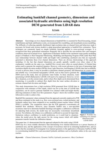
B. Fentie, Estimating bankfull channel geometry, dimensions and associated hydraulic attributes using highresolution DEM generated from LiDAR data2.3.Determination of bankfull channel dimensions and related hydraulic parametersWhilst it is beyond the scope of this paper, it may be possible to automate the determination of the point atwhich the bank will overflow. In this study the bankfull channel dimensions are determined by visuallyinspecting and deciding on a point on either side of the channel where flow over the bank would first occur.The bankfull width (Wbf) and bankfull depth/height (Hbf) are then determined as differences in horizontaldistance and height, respectively. In the example river channel profile shown in Figure 4 the bank wouldoverflow at the point shown on the right-hand-side of the channel at coordinate (242, 37). The correspondingpoint on the left-hand-side of the channel is at (98, 37). These two points determine the top width of the channelat bankfull. The lowest point at the channel bed is at (184, 22). One of the limitations of the topographic LiDARused in this study is that it does not include the depth of water in the channel at the time of LiDAR acquisition.This is clearly seen in Figure 4 where the bottom of the channel has roughly a constant elevation. Therefore, itis critical to estimate the flow depth at that time and subtract it from the elevation of the water surface in orderto determine the elevation of the stream bed.From the three coordinates representing bankfull height on either side of the channel and the thalweg in Figure4, determined above, it follows that:Hbf 37-22 2 17 mWbf 242-98 144 mwhere the 2 metres added in calculating Hbf is the estimated water depth at the time of LiDAR acquisition inthis study.Hydraulic radius is calculated 𝑝Where Area is cross-sectional area of flow and Wp is wetted perimeter.𝑅𝑅𝑏𝑏𝑏𝑏 5550Elevation (m)If a rectangular channel geometry is to be assumed, it would be necessary toconvert the channel dimensions determined above to equivalent rectangularchannel dimensions with the same hydraulic radius and bank height. With theseassumptions, the width of the equivalent rectangular rill (Wrec) is calculated fromthe equation for hydraulic radius ���𝑟𝑟 𝑅𝑅𝑏𝑏𝑏𝑏(2)1 𝐻𝐻𝑏𝑏𝑏𝑏Bankfull flow velocity (Vbf) is proportional to Rbf and is calculated from Manning’sequation as:𝑆𝑆 1/2,(3)𝑉𝑉𝑏𝑏𝑏𝑏 𝑅𝑅𝑏𝑏𝑏𝑏 2/3𝑛𝑛where S is channel bed slope, and n is Manning’s coefficient.Feature Profile 360(1)454098, 3735242, 37302520184, 220200400Distnace along the transect (m)Figure 4. An examplecross-section profile(Transect 3 in Fig.2)with the wettedperimeter at bankfullflow in shown in red.Bankfull discharge (Qbf) is then calculated as the product of bankfull cross-sectional area (Abf) and bankfullflow velocity (Vbf), or as:𝑄𝑄𝑏𝑏𝑏𝑏 𝐴𝐴𝑏𝑏𝑏𝑏 𝑉𝑉𝑏𝑏𝑏𝑏where Abf and Vbf are calculated from Equations 7 and 3.(4)The wetted perimeter at bankfull flow (Wp) is determined by summing the length along the bank at bankfullflow and the width of the channel bed. The length of each line segment is calculated from the PythagoreanTheorem as:(5)𝐿𝐿𝑖𝑖 (𝑦𝑦𝑖𝑖 𝑦𝑦𝑖𝑖 1 )2 (𝑥𝑥𝑖𝑖 𝑥𝑥𝑖𝑖 1 )2 ,where Li length of line segment i (i.e., each straight line in red in Figure 4), yi and xi are vertical distance(height) and horizontal distance respectively of line segment i.The wetted perimeter at bankfull (Wpbf) is then calculated from:𝑛𝑛𝑊𝑊𝑝𝑝𝑝𝑝𝑝𝑝 𝐿𝐿𝑖𝑖 .𝑖𝑖 11101(6)
B. Fentie, Estimating bankfull channel geometry, dimensions and associated hydraulic attributes using highresolution DEM generated from LiDAR dataSince the resolution of the DEM used in this study is 1 metre, 𝑥𝑥𝑖𝑖 𝑥𝑥𝑖𝑖 1 in Eq. 5 is also equal to 1, and thewetted perimeter in the example given in Figure 4 is composed of a total of 144 segments (i.e., n 144).The hydraulic radius at bankfull flow (Rbf) is calculated as the ratio of flow cross-sectional area at bankfullflow to wetted perimeter at bankfull flow. From the bankfull flow cross-section given in Figure 4, the area ofbankfull flow (Abf) can be calculated as:𝐴𝐴𝑏𝑏𝑏𝑏 Ar Auc ,(7)where:Ar 𝐸𝐸𝑏𝑏𝑏𝑏 𝑊𝑊bf ,(8)Ebf and Wbf are elevation and top width of channel at bankfull flow. Auc is the area under the curve definingthe channel at bankfull flow. This can be calculated using the trapezoidal rule as:𝐴𝐴𝑢𝑢𝑢𝑢 𝑛𝑛 1 𝑥𝑥 𝑥𝑥 𝑦𝑦0 𝑦𝑦𝑛𝑛 2(𝑦𝑦1 𝑦𝑦2 𝑦𝑦𝑛𝑛 1 ) 𝑦𝑦 𝑦𝑦𝑛𝑛 2𝑦𝑦𝑖𝑖 ,2 02(9)𝑖𝑖 1where x xi - xi-1 is resolution of the LiDAR DEM. Since the LiDAR DEM has a resolution of 1 metre, x 1. Therefore, the above equation simplifies to:𝐴𝐴𝑢𝑢𝑢𝑢𝑛𝑛 11 𝑦𝑦0 𝑦𝑦𝑛𝑛 2 𝑦𝑦𝑖𝑖 .2(10)𝑖𝑖 1It is, therefore, possible to use Eq. 4 to determine bankfull discharge given Wbf and Hbf instead of bankfull flowof a user specified recurrence interval currently adopted in P2R’s population of Dynamic SedNet parameters.It should be noted that the above formulae do not include depth of flow at the time of LiDAR data acquisition,as stated earlier in this paper. For the dataset used in this study flow depth was quite low at about 2 metres.Therefore, in the calculations for Table 1, it was assumed that the flow had a rectangular cross-section with awidth equal to the width of the water surface and awtdepth of 2 metres.RESULTS AND DISCUSSIONdwb20181614121086420Rrect (Wt Wb 600, d 20)Rtrap (Wb 400,Wt 600, d 20) Rtrap (Wb 100,Wt 600, d 20)Figure 5. Top: Hypothetical trapezoidal channel crosssection; Bottom: Comparison of hydraulic radiiassuming a rectangular channel against those oftrapezoidal cross-section (dimensions not to scale)Figure 6 depicts the river channel cross-sectionalprofile at the Miva gauging station. Channel widthand height (above the water surface) at bankfulldischarge as determined from the labelled coordinates on either side of thechannel are 176 (i.e., 266-90) metres and 13 (i.e., 32-19) metres, respectively.Figure 7, which has been generated from the Queensland government’s toring.information.qld.gov.au/), shows the flow level at the Miva gaugingstation between 2004 and 2019. This figure shows that the average flow depthduring the LiDAR acquisition period (17/07/2009 to 25/09/2009) is about 2metres and is among the lowest during that 2004-2019 period. Therefore, addingthe 2 metres water depth to the 13 metres height determined from Figure 7 givesus a bankfull height of 15 metres at this location. This is in agreement with andcorresponding to the value at the point of inflection (with a discharge of about2000 m3/s) from the stage-discharge rating curve produced by the QueenslandGovernment’s Water Monitoring Information Portal (Binns, 2016).110245403590, 3230Elevaion (m)Figure 5 depicts how hydraulic radius assuming arectangular channel is deviating from that of atrapezoidal channel (Rtrap) as its bottom width Wbdecreases from 400 to 100 metres while the topwidth Wt is kept constant at 600 metres with depth(d) assumed to be 20 metres. Figure 5 clearly showshow hydraulic radius and hence flow velocity anddischarge would be overestimated when atrapezoidal channel is assumed to be a rectangularone with width equal to bankfull width (Wbf) andbankfull height (Hbf) as in the P2R application ofDynamic SedNet.Hydraulic radius (m)3.266, 32252015163, 191050050100150200Distance along transect (m)250300Figure 6. Cross-sectionalprofile at the Miva station
B. Fentie, Estimating bankfull channel geometry, dimensions and associated hydraulic attributes using highresolution DEM generated from LiDAR dataAs outlined earlier, the profile graph data generated in ArcGIS is exported to a CSV file for generating a profilegraph of stream channel cross-section at each transect. A total of 52 channel cross-section profiles have beengenerated (20 on SC #636, and the other 32 on SC #489). Channel dimensions and hydraulic parameters atbankfull including depth (Hbf), width (Wbf), flow cross-sectional area (Abf), wetted perimeter (Wpbf), andhydraulic radius (Rbf) are calculated using equations that have been included in the Methods section.30Flow level (m)25Period of LiDAR capture (17/07/2009 - ure 7. Historical daily flow level (m) at the Miva gauging station where the low flow depth duringLiDAR data acquisition is highlighted in redAverage channel attributes at bankfull flow in the Dynamic SedNet model and corresponding valuesdetermined from the current study for each of the two modelled links are shown in Table 1. It is evident thatchannel attribute values in the Dynamic SedNet model are higher than the corresponding values determinedfrom the current study. For example, the link for SC #489 has a bankfull height of 21 m in the DynamicSedNet/Source model and only 12 as determined from this study. Given the high senstivity of the model tochanges in these parmaters (e.g., according to the author’s unpublished data, a 10% change in bankfull heightresults in about a 6% change in fine sediment export from this particular river system), it is crucial toestimate these parameters accurately. Therefore, although the Dynamic SedNet/ model has the capacity toadjust modelled erosion and floodplain deposition through calibration coefficients, overestimation of channelattributes leads to unrealistic model calibrated parameter values.Table 1. Average values of some flow parameters at bankfull flow for two modelled subcachments estimatedfrom this study against those applied in the current Dynamic SedNet 346145724915317100.0006644329323242142188412SC 071163020DynamicSedNetLiDAR21DynamicSedNetSC #636DynamicSedNetLiDARQ bf (m3/s)DynamicSedNetV bf (m/s)LiDARR bf (m)DynamicSedNetWpbf (m)LiDARA bf (m2)DynamicSedNetW bf (m)LiDARHbf (m)It can be seen from Figure 7 that, with the exception of one case, each of the 52 hydraulic radii determinedassuming irregular channel geometry in this study is less than the corresponding value determined assumingrectangular channel geometry. Therefore, hydraulic radius and hence stream power calculated using broad datainputs and regional relationships as a function of contributing area are typically overestimated as the result ofoverestimations in Wbf and Hbf (Table 1), and further compounded by the assumption of rectangular riverchannel geometry in these models as shown in Figure 8.4.CONCLUSIONStreambank retreat rate (RR) and floodplain deposition of fine sediment (FDfs) are two model components inDynamic SedNet that require bankfull flow as input. A method for deriving river channel dimensions andassociated hydraulic parameters from LiDAR water surface levels and flow level at the time of data acquisitionis developed and applied in the Mary catchment. The method allows visual estimation of bankfull height andwidth followed by calculation of other bankfull hydraulic parameters such as flow cross-sectional area (Abf),wetted perimeter (Wpbf), hydraulic radius (Rbf) as well as bankfull discharge (Qbf) and ultimately modellingstreambank erosion.1103
B. Fentie, Estimating bankfull channel geometry, dimensions and associated hydraulic attributes using highresolution DEM generated from LiDAR dataIn summary, this analysis has shown that, where LiDAR datais available, alternative approaches to determining criticalbank erosion parameters could be combined with existingknowledge of river systems to better inform broad scale waterquality models.ACKNOWLEDGEMENTSR assuming rectangular channell geometry (m)The study has:1. demonstrated that river channel dimensions and associated hydraulic attributes are more reliablydetermined from the use of LiDAR DEMs than by the approach typically adopted to informcatchment scale streambank erosion models (e.g., application of Dynamic SedNet in P2R),142. shown that the assumption of rectangular riverchannel geometry in the P2R application of Dynamic12SedNet is overestimating bankfull flow and10associated hydraulic attributes such as hydraulicradius and bankfull flow in the case study reaches,8and1: 1 line3. demonstrated that, where it is available, application6of LiDAR DEM may be a more reliable alternative4to the application of the concept of recurrenceinterval in estimating bankfull flow.20024681012R assuming irregular channell geometry (m)14Figure 8. Hydraulic radius (R) assumingirregular channel geometry vs thatassuming rectangular channel geometryI acknowledge that the LiDAR DEM used in this paper was provided by Peter Binns (formerly of theDepartment of Natural Resources, Mines and Energy) who has also given feedback on potential limitations ofthe data for the current study, which have been listed in the paper.REFERENCESBicknell, B.R., Imhoff, J.C., Kittle, J.L., Jobes, T.H., and Donigian, A.S. (2001). Hydrological SimulationProgram-Fortran: HSPF Version 12 Users Manual. U.S. Environmental Protection Agency, Athens,Georgia.Binns, P. (2016). Chronosequence mapping of streambank erosion: Mary River – Wide Bay Creek to MunnaCreek. State of QueenslandBinns, P. (2017). Use of remote imagery to verify modelled streambank retreat rates. MODIM2017, Hobart,Australia, 1906-1912sEllis, R.J. & Searle, R.D. (2014). ‘Dynamic SedNet Component Model Reference Guide: Concepts andalgorithms used in Source Catchments customisation plugin for Great Barrier Reef catchment modelling’.Queensland Department of Science, Information Technology, Innovation and the Arts, Bundaberg, Qld.Fisher, G. B., Bookhagen, B., Amos, C. B. (2013). Channel planform geometry and slopes from freely availablehigh-spatial resolution imagery and DEM fusion: Implications for channel width scaling, erosion proxies,and fluvial signatures in tectonically active landscapesHec-GeoRAS (US Army Corp of Engineers). /Legleiter, C. J. (2012). Remote measurement of river morphology via fusion of LiDAR topography andspectrally based bathymetry. Earth Surf. Process. Landforms 37, 499–518McKean, J., Nagel, D., Tonina, D., Bailey, P., Wright, C.W., Bohn, C., Nayegandhi, A. (2009). Remote sensingof channels and riparian zones with a narrow-beam aquatic-terrestrial lidar. Remote Sensing, 1, 1065-1096Narasimhan, B., Allen, P.M., Coffman, S.V., Arnold, J.G. and Srinivasan, R. (2017). Development and Testingof a Physically Based Model of Streambank Erosion for Coupling with a Basin-Scale Hydrologic ModelSWAT. Journal of the American Water Resources Association (JAWRA) 53(2):344-364. DOI:10.1111/1752-1688.12505Roux, C., Alber, A., Bertrand, M., Vaudor, L., Piégay, H. (2015), “FluvialCorridor”: A new ArcGIS toolboxpackage for multiscale riverscape exploration. Geomorphology 242, 29–37Schumann, G., Matgen P., Cutler, M.E.J., Black, A., Hoffmann, L., Pfister, L. (2008). Comparison of remotelysensed water stages from LiDAR, topographic contours and SRTM. ISPRS Journal of Photogrammetry &Remote Sensing 63 (2008) 283–296Smart, G.M., Bind J. Duncan, M.J. (2009). River bathymetry from conventional LiDAR using water surfacereturns. 18th World IMACS / MODSIM Congress, Cairns, Australia 13-17Wilkinson, S.N., C. Dougall, A.E. Kinsey-Henderson, R.D. Searle, R.J. Ellis, and R. Bartley, 2013.Development of a Time-Stepping Sediment Budget Model for Assessing Land Use Impacts in Large RiverBasins. Science of the Total Environment 468–469:1210-1224, DOI: 10.1016/j.scitoenv.2013.07.049.1104
Application of Dynamic SedNet in the catchment water quality modelling project of Paddock to Reef Integrated Monitoring, Modelling and Reporting Program (P2R) under Reef Plan uses relationships between channel width and height with contributing catchment area that are regionally generated to determine these river channel dimensions.