Transcription
What to Do about Missing Values in Time-SeriesCross-Section DataJames Honaker The Pennsylvania State UniversityGary King Harvard UniversityApplications of modern methods for analyzing data with missing values, based primarily on multiple imputation, have inthe last half-decade become common in American politics and political behavior. Scholars in this subset of political sciencehave thus increasingly avoided the biases and inefficiencies caused by ad hoc methods like listwise deletion and best guessimputation. However, researchers in much of comparative politics and international relations, and others with similar data,have been unable to do the same because the best available imputation methods work poorly with the time-series crosssection data structures common in these fields. We attempt to rectify this situation with three related developments. First, webuild a multiple imputation model that allows smooth time trends, shifts across cross-sectional units, and correlations overtime and space, resulting in far more accurate imputations. Second, we enable analysts to incorporate knowledge from areastudies experts via priors on individual missing cell values, rather than on difficult-to-interpret model parameters. Third,because these tasks could not be accomplished within existing imputation algorithms, in that they cannot handle as manyvariables as needed even in the simpler cross-sectional data for which they were designed, we also develop a new algorithmthat substantially expands the range of computationally feasible data types and sizes for which multiple imputation can beused. These developments also make it possible to implement the methods introduced here in freely available open sourcesoftware that is considerably more reliable than existing algorithms.We develop an approach to analyzing data withmissing values that works well for large numbers of variables, as is common in Americanpolitics and political behavior; for cross-sectional, timeseries, or especially “time-series cross-section” (TSCS)data sets (i.e., those with T units for each of N crosssectional entities such as countries, where often T N),as is common in comparative politics and internationalrelations; or for when qualitative knowledge exists aboutspecific missing cell values. The new methods greatly increase the information researchers are able to extract fromgiven amounts of data and are equivalent to having muchlarger numbers of observations available.Our approach builds on the concept of “multipleimputation,” a well-accepted and increasingly commonapproach to missing data problems in many fields. Theidea is to extract relevant information from the observedportions of a data set via a statistical model, to imputemultiple (around five) values for each missing cell, andto use these to construct multiple “completed” data sets.In each of these data sets, the observed values are thesame, and the imputations vary depending on the estimated uncertainty in predicting each missing value. Thegreat attraction of the procedure is that after imputation,analysts can apply to each of the completed data sets whatever statistical method they would have used if there hadbeen no missing values and then use a simple procedureto combine the results. Under normal circumstances, researchers can impute once and then analyze the imputeddata sets as many times and for as many purposes as theywish. The task of running their analyses multiple timesand combining results is routinely and transparentlyJames Honaker is a lecturer at The Pennsylvania State University, Department of Political Science, Pond Laboratory, University Park, PA16802 (tercer@psu.edu). Gary King is Albert J. Weatherhead III University Professor, Harvard University, Institute for Quantitative SocialScience, 1737 Cambridge Street, Cambridge, MA 02138 (king@harvard.edu, http://gking.harvard.edu).All information necessary to replicate the results in this article can be found in Honaker and King (2010). We have written an easy-to-usesoftware package, with Matthew Blackwell, that implements all the methods introduced in this article; it is called “Amelia II: A Programfor Missing Data” and is available at http://gking.harvard.edu/amelia. Our thanks to Neal Beck, Adam Berinsky, Matthew Blackwell, JeffLewis, Kevin Quinn, Don Rubin, Ken Scheve, and Jean Tomphie for helpful comments, the National Institutes of Aging (P01 AG17625-01),the National Science Foundation (SES-0318275, IIS-9874747, SES-0550873), and the Mexican Ministry of Health for research support.American Journal of Political Science, Vol. 54, No. 2, April 2010, Pp. 561–581 C 2010,Midwest Political Science AssociationISSN 0092-5853561
JAMES HONAKER AND GARY KING562handled by special purpose statistical analysis software.As a result, after careful imputation, analysts can ignorethe missingness problem (King et al. 2001; Rubin 1987).Commonly used multiple imputation methods workwell for up to 30–40 variables from sample surveys andother data with similar rectangular, nonhierarchical properties, such as from surveys in American politics orpolitical behavior where it has become commonplace.However, these methods are especially poorly suited todata sets with many more variables or the types of dataavailable in the fields of political science where missingvalues are most endemic and consequential, and wheredata structures differ markedly from independent drawsfrom a given population, such as in comparative politicsand international relations. Data from developing countries especially are notoriously incomplete and do notcome close to fitting the assumptions of commonly usedimputation models. Even in comparatively wealthy nations, important variables that are costly for countries tocollect are not measured every year; common examplesused in political science articles include infant mortality,life expectancy, income distribution, and the total burdenof taxation.When standard imputation models are applied toTSCS data in comparative and international relations,they often give absurd results, as when imputations inan otherwise smooth time series fall far from previous and subsequent observations, or when imputed values are highly implausible on the basis of genuine localknowledge. Experiments we have conducted where selected observed values are deleted and then imputed withstandard methods produce highly uninformative imputations. Thus, most scholars in these fields eschew multipleimputation. For lack of a better procedure, researcherssometimes discard information by aggregating covariatesinto five- or ten-year averages, losing variation on the dependent variable within the averages (see, for example,Iversen and Soskice 2006; Lake and Baum 2001; Moeneand Wallerstein 2001; and Timmons 2005, respectively).Obviously this procedure can reduce the number of observations on the dependent variable by 80 or 90%, limitsthe complexity of possible functional forms estimatedand number of control variables included, due to therestricted degrees of freedom, and can greatly affect empirical results—a point regularly discussed and lamentedin the cited articles.These and other authors also sometimes develop adhoc approaches such as imputing some values with linear interpolation, means, or researchers’ personal bestguesses. These devices often rest on reasonable intuitions:many national measures change slowly over time, observations at the mean of the data do not affect inferences forsome quantities of interest, and expert knowledge outsidetheir quantitative data set can offer useful information. Toput data in the form that their analysis software demands,they then apply listwise deletion to whatever observationsremain incomplete. Although they will sometimes workin specific applications, a considerable body of statistical literature has convincingly demonstrated that thesetechniques routinely produce biased and inefficient inferences, standard errors, and confidence intervals, and theyare almost uniformly dominated by appropriate multipleimputation-based approaches (Little and Rubin 2002).1Applied researchers analyzing TSCS data must thenchoose between a statistically rigorous model of missingness, predicated on assumptions that are clearly incorrectfor their data and which give implausible results, or ad hocmethods that are known not to work in general but whichare based implicitly on assumptions that seem more reasonable. This problem is recognized in the comparativepolitics literature where scholars have begun to examinethe effect of missing data on their empirical results. Forexample, Ross (2006) finds that the estimated relationship between democracy and infant mortality depends onthe sample that remains after listwise deletion. Timmons(2005) shows that the relationship found between taxation and redistribution depends on the choice of taxationmeasure, but superior measures are subject to increasedmissingness and so not used by researchers. And Spence(2007) finds that Rodrik’s (1998) results are dependenton the treatment of missing data.We offer an approach here aimed at solving theseproblems. In addition, as a companion to this article,we make available (at http://gking.harvard.edu/amelia)1King et al. (2001) show that, with the average amount of missingness evident in political science articles, using listwise deletionunder the most optimistic of assumptions causes estimates to beabout a standard error farther from the truth than failing to control for variables with missingness. The strange assumptions thatwould make listwise deletion better than multiple imputation areroughly that we know enough about what generated our observeddata to not trust them to impute the missing data, but we stillsomehow trust the data enough to use them for our subsequentanalyses. For any one observation, the misspecification risk fromusing all the observed data and prior information to impute afew missing values will usually be considerably lower than the riskfrom inefficiency that will occur and selection bias that may occur when listwise deletion removes the dozens of more numerousobserved cells. Application-specific approaches, such as models forcensoring and truncation, can dominate general-purpose multiple imputation algorithms, but they must be designed anew foreach application type, are unavailable for problems with missingness scattered throughout an entire data matrix of dependent andexplanatory variables, and tend to be highly model-dependent. Although these approaches will always have an important role to playin the political scientist’s toolkit, since they can also be used together with multiple imputation, we focus here on more widelyapplicable, general-purpose algorithms.
WHAT TO DO ABOUT MISSING VALUESan easy-to-use software package that implements all themethods discussed here. The software, called Amelia II: AProgram for Missing Data, works within the R Project forStatistical Computing or optionally through a graphicaluser interface that requires no knowledge of R (Honaker,King, and Blackwell 2009). The package also includesdetailed documentation on implementation details, howto use the method in real data, and a set of diagnostic routines that can help evaluate when the methodsare applicable in a particular set of data. The nature ofthe algorithms and models developed here makes thissoftware faster and more reliable than existing imputation packages (a point which statistical software reviews have already confirmed; see Horton and Kleinman2007).Multiple Imputation ModelMost common methods of statistical analysis require rectangular data sets with no missing values, but data setsfrom the real political world resemble a slice of swisscheese with scattered missingness throughout. Considerable information exists in partially observed observationsabout the relationships between the variables, but listwisedeletion discards all this information. Sometimes this isthe majority of the information in the original data set.2Continuing the analogy, what most researchers tryto do is to fill in the holes in the cheese with varioustypes of guesses or statistical estimates. However, unlessone is able to fill in the holes with the true values ofthe data that are missing (in which case there would beno missing data), we are left with “single imputations”which cause statistical analysis software to think the datahave more observations than were actually observed andto exaggerate the confidence you have in your results bybiasing standard errors and confidence intervals.That is, if you fill the holes in the cheese with peanutbutter, you should not pretend to have more cheese! Analysis would be most convenient for most computer programs if we could melt down the cheese and reform itinto a smaller rectangle with no holes, adding no new information, and thus not tricking our computer program2If archaeologists threw away every piece of evidence, every tablet,every piece of pottery that was incomplete, we would have entirecultures that disappeared from the historical record. We would nolonger have the Epic of Gilgamesh, or any of the writings of Sappho.It is a ridiculous proposition because we can take all the partialsources, all the information in each fragment, and build themtogether to reconstruct much of the complete picture without anyinvention. Careful models for missingness allow us to do the samewith our own fragmentary sources of data.563into thinking there exists more data than there really is.Doing the equivalent, by filling in observations and thendeleting some rows from the data matrix, is too difficult to do properly; and although methods of analysisadapted to the swiss cheese in its original form exist (e.g.,Heckman 1990; King et al. 2004), they are mostly notavailable for missing data scattered across both dependent and explanatory variables.Instead, what multiple imputation does is to fill inthe holes in the data using a predictive model that incorporates all available information in the observed datatogether along with any prior knowledge. Separate “completed” data sets are created where the observed dataremain the same, but the missing values are “filled in”with different imputations. The “best guess” or expectedvalue for any missing value is the mean of the imputedvalues across these data sets; however, the uncertaintyin the predictive model (which single imputation methods fail to account for) is represented by the variationacross the multiple imputations for each missing value.Importantly, this removes the overconfidence that wouldresult from a standard analysis of any one completeddata set, by incorporating into the standard errors of ourultimate quantity of interest the variation across our estimates from each completed data set. In this way, multiple imputation properly represents all information ina data set in a format more convenient for our standard statistical methods, does not make up any data, andgives accurate estimates of the uncertainty of any resultinginferences.We now describe the predictive model used mostoften to generate multiple imputations. Let D denote avector of p variables that includes all dependent and explanatory variables to be used in subsequent analyses,and any other variables that might predict the missingvalues. Imputation models are predictive and not causaland so variables that are posttreatment, endogenously determined, or measures of the same quantity as others canall be helpful to include as long as they have some predictive content. In particular, including the dependentvariable to impute missingness in an explanatory variableinduces no endogeneity bias, and randomly imputing anexplanatory variable creates no attenuation bias, becausethe imputed values are drawn from the observed dataposterior. The imputations are a convenience for the analyst because they rectangularize the data set, but theyadd nothing to the likelihood and so represent no newinformation even though they enable the analyst to avoidlistwise deleting any unit that is not fully observed on allvariables.We partition D into its observed and missing elements, respectively: D {D obs , D mis }. We also define a
564missingness indicator matrix M (with the same dimensions as D) such that each element is a 1 if the corresponding element of D is missing and 0 if observed. Theusual assumption in multiple imputation models is thatthe data are missing at random (MAR), which means thatM can be predicted by D obs but not (after controlling forD obs ) D mis , or more formally p(M D) p(M D obs ).MAR is related to the assumptions of ignorability, nonconfounding, or the absence of omitted variable bias thatare standard in most analysis models. MAR is much saferthan the more restrictive missing completely at random(MCAR) assumption which is required for listwise deletion, where missingness patterns must be unrelated toobserved or missing values: P (M D) P (M). MCARwould be appropriate if coin flips determined missingness, whereas MAR would be better if missingness mightalso be related to other variables, such as mortality datanot being available during wartime. An MAR assumptioncan be wrong, but it would by definition be impossibleto know on the basis of the data alone, and so all existinggeneral-purpose imputation models assume it. The keyto improving a multiple imputation model is includingmore information in the model so that the stringency ofthe ignorability assumption is lessened.An approach that has become standard for the widestrange of uses is based on the assumption that D is multivariate normal, D N( , ), an implication of whichis that each variable is a linear function of all others.Although this is an approximation, and one not usually appropriate for analysis models, scholars have shownthat for imputation it usually works as well as more complicated alternatives designed specially for categorical ormixed data (Schafer 1997; Schafer and Olsen 1998). Allthe innovations in this article would easily apply to thesemore complicated alternative models, but we focus on thesimpler normal case here. Furthermore, as long as the imputation model contains at least as much information asthe variables in the analysis model, no biases are generatedby introducing more complicated models (Meng 1994). Infact, the two-step nature of multiple imputation has twoadvantages over “optimal” one-step approaches. First, including variables or information in the imputation modelnot needed in the analysis model can make estimates evenmore efficient than a one-step model, a property knownas “super-efficiency.” And second, the two-step approachis much less model-dependent because no matter howbadly specified the imputation model is, it can only affectthe cell values that are missing.Once m imputations are created for each missingvalue, we construct m completed data sets and run whatever procedure we would have run if all our data hadbeen observed originally. From each analysis, a quantityJAMES HONAKER AND GARY KINGof interest is computed (a descriptive feature, causal effect, prediction, counterfactual evaluation, etc.) and theresults are combined. The combination can follow Rubin’s (1987) original rules, which involve averaging thepoint estimates and using an analogous but slightly moreinvolved procedure for the standard errors, or more simply by taking 1/m of the total required simulations ofthe quantities of interest from each of the m analysesand summarizing the set of simulations as is now common practice with single models (e.g., King, Tomz, andWittenberg 2000).Computational Difficulties andBootstrapping SolutionsA key computational difficulty in implementing the normal multiple imputation algorithm is taking randomdraws of and from their posterior densities in orderto represent the estimation uncertainty in the problem.One reason this is hard is that the p( p 3)/2 elementsof and increase rapidly with the number of variablesp. So, for example, a problem with only 40 variables has860 parameters and drawing a set of these parameters atrandom requires inverting an 860 860 variance matrixcontaining 370,230 unique elements.Only two statistically appropriate algorithms arewidely used to take these draws. The first proposed is theimputation-posterior (IP) approach, which is a Markovchain, Monte Carlo–based method that takes both expertise to use and considerable computational time. Theexpectation maximization importance sampling (EMis)algorithm is faster than IP, requires less expertise, andgives virtually the same answers. See King et al. (2001)for details of the algorithms and citations to those whocontributed to their development. Both EMis and IP havebeen used to impute many thousands of data sets, butall software implementations have well-known problemswith large data sets and TSCS designs, creating unacceptably long run-times or software crashes.We approach the problem of sampling and bymixing theories of inference. We continue to use Bayesiananalysis for all other parts of the imputation process andto replace the complicated process of drawing and from their posterior density with a bootstrapping algorithm. Creative applications of bootstrapping have beendeveloped for several application-specific missing dataproblems (Efron 1994; Lahlrl 2003; Rubin 1994; Rubinand Schenker 1986; Shao and Sitter 1996), but to ourknowledge the technique has not been used to developand implement a general-purpose multiple imputationalgorithm.
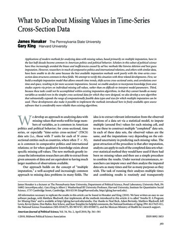
WHAT TO DO ABOUT MISSING VALUESThe result is conceptually simple and easy to implement. Whereas EMis and especially IP are elaborate algorithms, requiring hundreds of lines of computer codeto implement, bootstrapping can be implemented in justa few lines. Moreover, the variance matrix of and need not be estimated, importance sampling need notbe conducted and evaluated (as in EMis), and Markovchains need not be burnt in and checked for convergence(as in IP). Although imputing much more than about40 variables is difficult or impossible with current implementations of IP and EMis, we have successfully imputedreal data sets with up to 240 variables and 32,000 observations; the size of problems this new algorithm can handleappears to be constrained only by available memory. Webelieve it will accommodate the vast majority of appliedproblems in the social sciences.Specifically, our algorithm draws m samples of size nwith replacement from the data D.3 In each sample, werun the highly reliable and fast EM algorithm to producepoint estimates of and (see the appendix for a description). Then for each set of estimates, we use the originalsample units to impute the missing observations in theiroriginal positions. The result is m multiply imputed datasets that can be used for subsequent analyses.Since our use of bootstrapping meets standard regularity conditions, the bootstrapped estimates of and have the right properties to be used in place of drawsfrom the posterior. The two are very close empirically inlarge samples (Efron 1994). In addition, bootstrappinghas better lower order asymptotics than the parametricapproaches IP and EMis implement. Just as symmetryinducing transformations (like ln( 2 ) in regression problems) make the asymptotics kick in faster in likelihoodmodels, it may then be that our approach will more faithfully represent the underlying sampling density in smallersamples than the standard approaches, but this should beverified in future research.43This basic version of the bootstrap algorithm is appropriate whensufficient covariates are included (especially as described in thefourth section) to make the observations conditionally independent. Although we have implemented more sophisticated bootstrapalgorithms for when conditional independence cannot be accomplished by adding covariates (Horowitz 2001), we have thus far notfound them necessary in practice.4Extreme situations, such as small data sets with bootstrapped samples that happen to have constant values or collinearity, should notbe dropped (or uncertainty estimates will be too small) but are easily avoided via the traditional use of empirical (or “ridge”) priors(Schafer 1997, 155).The usual applications of bootstrapping outside the imputationcontext requires hundreds of draws, whereas multiple imputationonly requires five or so. The difference has to do with the amount ofmissing information. In the usual applications, 100% of the parameters of interest are missing, whereas for imputation, the fraction565The already fast speed of our algorithm can be increased by approximately m 100% because our algorithm has the property that computer scientists call“embarrassingly parallel,” which means that it is easy tosegment the computation into separate, parallel processeswith no dependence among them until the end. In a parallel environment, our algorithm would literally finishbefore IP begins (i.e., after starting values are computed,which are typically done with EM), and about at the pointwhere EMis would be able to begin to utilize the parallelenvironment.We now replicate the “MAR-1” Monte Carlo experiment in King et al. (2001, 61), which has 500 observationsand about 78% of the rows fully observed. This simulation was developed to show the near equivalence of resultsfrom EMis and IP, and we use it here to demonstrate thatthose results are also essentially equivalent to our newbootstrapped-based EM algorithm. Figure 1 plots theestimated posterior distribution of three parameters forour approach (labeled EMB), IP/EMis (for which only oneline was plotted because they were so close), the completedata with the true values included, and listwise deletion.For all three graphs in the figure, one for each parameter,IP, EMis, and EMB all give approximately the same result.The distribution for the true data is also almost the same,but slightly more peaked (i.e., with smaller variance), asshould be the case since the simulated observed data without missingness have more information. IP has a smallervariance than EMB for two of the parameters and largerfor one; since EMB is more robust to distributional andsmall sample problems, it may well be more accurate herebut in any event they are very close in this example. The(red) listwise deletion density is clearly biased away fromthe true density with the wrong sign, and much largervariance.Trends in Time, Shifts in SpaceThe commonly used normal imputation model assumesthat the missing values are linear functions of other variables’ observed values, observations are independent conditional on the remaining observed values, and all theobservations are exchangable in that the data are not organized in hierarchical structures. These assumptions haveof cells in a data matrix that are missing is normally considerablyless than half. For problems with much larger fractions of missinginformation, m will need to be larger than five but rarely anywherenear as large as would be required for the usual applications ofbootstrapping. The size of m is easy to determine by merely creating additional imputed data sets and seeing whether inferenceschange.
JAMES HONAKER AND GARY KING566FIGURE 1Histograms Representing PosteriorDensities from Monte CarloSimulated Data (n 500 and about78% of the Units Fully Observed), viaThree Algorithms and the Complete(Normally Unobserved) Dataβ0 0.4 0.20.0β10.20.4 0.4 0.20.00.20.4β2EMBIP EMisComplete DataList wise Del. 0.4 0.20.00.20.4IP and EMis, and our algorithm (EMB) are very close in all threegraphs, whereas listwise deletion is notably biased with highervariance.proven to be reasonable for survey data, but they clearlydo not work for TSCS data. In this section and the next,we take advantage of these discrepancies to improve imputations by adapting the standard imputation model,with our new algorithm, to reflect the special nature ofthese data. Most critically in TSCS data, we need to recognize the tendency of variables to move smoothly overtime, to jump sharply between some cross-sectional unitslike countries, to jump less or be similar between somecountries in close proximity, and for time-series patternsto differ across many countries.5 We discuss smoothnessover time and shifts across countries in this section and5The closest the statistical literature on missing data has come totackling TSCS data would seem to be “repeated measures” designs,where clinical patients are observed over a small number of irregularly spaced time intervals (Little 1995; Molenberghs and Verbeke2005). Missingness occurs principally in the dependent variable(the patient’s response to treatment) and largely due to attrition,leading to monotone missingness patterns. As attrition is often dueto a poor response to treatment, MAR is usually implausible and somissingness models are necessarily assumption-dependent (Davey,S̃hanahan, and Schafer 2001; Kaciroti et al. 2008). Since in typicalTSCS applications, missingness is present in all variables, and timeseries are longer, direct application of these models is infeasiblethen consider issues of prior information, nonignorability, and spatial correlation in the next.Many time-series variables, such as GDP, human capital, and mortality, change relatively smoothly over time.If an observation in the middle of a time series is missing, then the true value often will not deviate far from asmooth trend plotted through the data. The smooth trendneed not be linear, and so the imputation technique oflinear interpolation, even if modified to represent uncertainty appropriately, may not work. Moreover, sharpdeviations from a smooth trend may be caused by othervariables, such as a civil war. This same war might alsoexplain why the observation is missing. Such deviates willsometimes make linear interpolation badly biased, evenwhen accurate imputations can still be constructed basedon predictions using other variables in the data set (suchas the observed intensity of violence in the country).We include th
Gary King Harvard University Applications of modern methods for analyzing data with missing values, based primarily on multiple imputation, have in . This problem is recognized in the comparative politics literature where scholars have begun to examine the effect of missing data on their empirical results. For example, Ross (2006) finds that .