WIXLIB

Pattern Recognition and Machine LearningChapter 9: Mixture Models and EMThomas MensinkJakob VerbeekOctober 11, 2007Thomas Mensink, Jakob VerbeekBishop Chapter 9: Mixture Models and EM

Le Menu9.1 K-means clusteringGetting the idea with a simple example9.2 Mixtures of GaussiansGradient fixed-points & responsibilities9.3 An alternative view of EMCompleting the data with latent variables9.4 The EM algorithm in generalUnderstanding EM as coordinate ascentThomas Mensink, Jakob VerbeekBishop Chapter 9: Mixture Models and EM

Mixture Models and EM: IntroductionIAdditional latent variables allows to express relatively complexmarginal distributions over latent variables in terms of moretractable joint distributions over the expanded space.IMaximum-Likelihood estimator in such a space is theExpectation-Maximization (EM) algorithm.IChapter 10 provides Bayesian treatment using variationalinferenceThomas Mensink, Jakob VerbeekBishop Chapter 9: Mixture Models and EM

K-Means Clustering: Distortion MeasureIDataset {x1 , . . . , xN }IPartition in K clustersICluster prototype: µkIBinary indicator variable, 1-of-K Coding schemernk {0, 1}rnk 1, and rnj 0 for j 6 k.Hard assignment.IDistortion measureJ N XKXrnk kxn µk k2n 1 k 1Thomas Mensink, Jakob VerbeekBishop Chapter 9: Mixture Models and EM(9.1)

K-Means Clustering: Expectation MaximizationIFind values for {rnk } and {µk } to minimize:J N XKXrnk kxn µk k2(9.1)n 1 k 1IIterative procedure:1. Minimize J w.r.t. rnk , keep µk fixed (Expectation) 1 if k arg minj kxn µk k2rnk 0 otherwise(9.2)2. Minimize J w.r.t. µk , keep rnk fixed (Maximization)2NXrnk (xn µk ) 0(9.3)n 1Pn rnk xnµk Pn rnkThomas Mensink, Jakob VerbeekBishop Chapter 9: Mixture Models and EM(9.4)

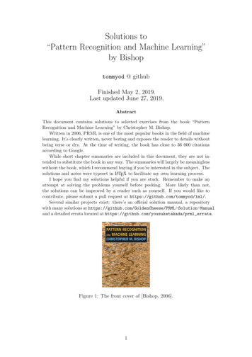
K-Means Clustering: Example2(a)2002(d)0 2 2202(e)02(g)002(h)020201234(i)0 2 21000500 220 22 2 220(f)0 2 2 220 2(c)0 2 2220 22(b) 2 202 202IEach E or M step reduces the value of the objective function JIConvergence to a global or local maximumThomas Mensink, Jakob VerbeekBishop Chapter 9: Mixture Models and EM

K-Means Clustering: Concluding remarks1. Direct implementation of K-Means can be slow2. Online version:oldµnew µoldkk ηn (xn µk )(9.5)3. K-mediods, general distortion measureJ N XKXrnk V(xn , µk )(9.6)n 1 k 1where V(·, ·) is any kind of dissimilarity measure4. Image segmentation and compression example: 4.2 %8.3 %Thomas Mensink, Jakob Verbeek16.7 %Original image100 %Bishop Chapter 9: Mixture Models and EM

Mixture of Gaussians: Latent variablesIGaussian Mixture Distribution:p(x) KXπk N (x µk , Σk )(9.7)k 1IIntroduce latent variable zzIz is binary 1-of-K coding variableIp(x, z) p(z)p(x z)Thomas Mensink, Jakob VerbeekxBishop Chapter 9: Mixture Models and EM

Mixture of Gaussians: Latent variables (2)Ip(zk 1) πkPconstraints:0 π 1,andkk πk 1Qp(z) k πkzkIp(x zk Q1) N (x µk , Σk )p(x z) k N (x µk , Σk )zkIp(x) IThe use of the joint probability p(x, z), leads to significantsimplificationsPzp(x, z) Pzp(z)p(x z) Thomas Mensink, Jakob VerbeekPkπk N (x µk , Σk )Bishop Chapter 9: Mixture Models and EM

Mixture of Gaussians: Latent variables (3)Iresponsibility of component k to generate observation x(9.13):p(zk 1)p(x zk 1)γ(zk ) p(zk 1 x) Pk p(zk 1)p(x zk 1)πk N (x µk , Σk ) Pk πk N (x µk , Σk )Iis the posterior probabilityGenerate random samples with ancestral sampling:First generate ẑ from p(z)Second generate a value for x from p(x ẑ)See Chapter 11.11(a)0.51(b)0.500.5000.51Thomas Mensink, Jakob Verbeek(c)000.5100.51Bishop Chapter 9: Mixture Models and EM

Mixture of Gaussians: Maximum LikelihoodznIπLog Likelihoodxnln p(X π, µ, Σ) NXn 1ln(KX)µπk N (x µk , Σk )ΣNk 1(9.14)ISingularity when a mixture componentcollapses on a datapointIIdentifiability for a ML solution in aK-component mixture there are K!equivalent solutions.p(x)xThomas Mensink, Jakob VerbeekBishop Chapter 9: Mixture Models and EM

Mixture of Gaussians: EM for Gaussian MixturesIIInformal introduction of expectation-maximization algorithm(Dempster et al., 1977).Maximum of log likelihood:derivatives of ln p(X π, µ, Σ) w.r.t parameters to 0.(K)NXXln p(X π, µ, Σ) lnπk N (x µk , Σk )(9.14)n 1Ik 1For the µk 1 :0 NXπ N (x µk , Σk )PkΣ 1k (xn µk )πN(x µ,Σ)kkkkn 1 {z}(9.16)γ(zk )X1γ(zk )xnn γ(zk ) nµk P1Error in book, see erata fileThomas Mensink, Jakob VerbeekBishop Chapter 9: Mixture Models and EM(9.17)

Mixture of Gaussians: EM for Gaussian MixturesIFor Σk :X1γ(zk )(xn µk )(xn µk )Tn γ(zk ) nΣk PI(9.19)For the πk :IITake into account constraintLagrange multiplierPkπk 1Xln p(X π, µ, Σ) λ(πk 1)(9.20)k0 XN (x µk , Σk ) λk πk N (x µk , Σk )Pγ(zk )πk nNPnThomas Mensink, Jakob VerbeekBishop Chapter 9: Mixture Models and EM(9.21)(9.22)

Mixture of Gaussians: EM for Gaussian Mixtures ExampleINo closed form solutions: γ(zk ) depends on parametersIBut these equations suggest simple iterative scheme forfinding maximum likelihood:Alternate between estimating the current γ(zk ) and updatingthe parameters {µk , Σk , πk }.222000 2 2 220(a)2 2 2 20(b)2 22000 2 2 2 20(d)2 20(e)20(c)20(f)2 2IMore iterations needed to converge than K-means algorithm,and each cycle requires more computationICommon, initialise parameters based K-means run.Thomas Mensink, Jakob VerbeekBishop Chapter 9: Mixture Models and EM

Mixture of Gaussians: EM for Gaussian Mixtures ExampleINo closed form solutions: γ(zk ) depends on parametersIBut these equations suggest simple iterative scheme forfinding maximum likelihood:Alternate between estimating the current γ(zk ) and updatingthe parameters {µk , Σk , πk }.222000 2 2 220(a)2 2 2 20(b)2 22000 2 2 2 20(d)2 20(e)20(c)20(f)2 2IMore iterations needed to converge than K-means algorithm,and each cycle requires more computationICommon, initialise parameters based K-means run.Thomas Mensink, Jakob VerbeekBishop Chapter 9: Mixture Models and EM

Mixture of Gaussians: EM for Gaussian Mixtures Summary1. Initialize {µk , Σk , πk } and evaluate log-likelihood2. E-Step Evaluate responsibilities γ(zk )3. M-Step Re-estimate paramters, using current responsibilities:X1γ(zk )xnn γ(zk ) nX1γ(zk )(xn µk )(xn µk )T Pγ(z)knnPγ(z)k nNµnew Pk(9.23)Σnewk(9.24)πknew4. Evaluate log-likelihood ln p(X π, µ, Σ) and check forconvergence (go to step 2).Thomas Mensink, Jakob VerbeekBishop Chapter 9: Mixture Models and EM(9.25)

An Alternative View of EM: latent variablesILet X observed data, Z latent variables, θ parameters.IGoal: maximize marginal log-likelihood of observed data()Xln p(X θ) lnp(X, Z θ) .(9.29)ZIOptimization problematic due to log-sum.IAssume straightforward maximization for complete dataln p(X, Z θ).ILatent Z is known only through p(Z X, θ).IWe will consider expectation of complete data log-likelihood.Thomas Mensink, Jakob VerbeekBishop Chapter 9: Mixture Models and EM

An Alternative View of EM: algorithmIInitialization: Choose initial set of parameters θold .IE-step: use current parameters θold to compute p(Z X, θold )to find expected complete-data log-likelihood for general θXQ(θ, θold ) p(Z X, θold ) ln p(X, Z θ).(9.30)ZIM-step: determine θnew by maximizing (9.30)θnew arg maxθ Q(θ, θold ).I(9.31)Check convergence: stop, or θold θnew and go to E-step.Thomas Mensink, Jakob VerbeekBishop Chapter 9: Mixture Models and EM

An Alternative View of EM: Gaussian mixtures revisitedIFor mixture assign each x latent assigment variables zk .IComplete-data (log-)likelihood (9.36), and expectation (9.40)p(x, z θ) ln p(x, z θ) Q(θ) IEz [ln p(x, z θ)] KYk 1KXk 1KXπkzk N (x; µk , Σk )zkzk {ln πk ln N (x; µk , Σk )}γ(zk ) {ln πk ln N (x; µk , Σk )}k 1zn1π1(a)0.5(c)0.5xnµΣN000Thomas Mensink, Jakob Verbeek0.5100.5Bishop Chapter 9: Mixture Models and EM1

Example EM algorithm: Bernoulli mixturesIBernoulli distributions over binary data vectorsp(x µ) DYµxi i (1 µi )(1 xi ) .(9.44)i 1IMixture of Bernoullis can model variable correlations.IAs the Gaussian, Bernoulli is member of exponential familyIImodel log-linear, mixture not, complete-data log-likelihood is.Simple EM algorithm to find ML parametersIIE-step: compute responsibilities γ(znk )P πk p(xn µk )M-step: updatePparameters πk N 1 n γ(znk ), andµk (N πk ) 1 n γ(znk )xnThomas Mensink, Jakob VerbeekBishop Chapter 9: Mixture Models and EM

Example EM algorithm: Bayesian linear regressionIRecall Bayesian linear regression: it’s a latent variable modelN YN tn ; w φ(xn ), β 1 , (3.10)p(t w, β, X) n 1 p(w α) N w; 0, α 1 I ,Zp(t α, β, X) p(t w, β)p(w α) dw.I(3.52)(3.77)Simple EM algorithm to find ML parameters (α, β)IE-step: compute responsibilities over latent variable wp(w t, α, β) N (w; m, S) ,Im βSΦ t,S 1 αI βΦ Φ.M-step: update parameters using complete-data log-likelihoodα 1 (1/M ) m m Tr{S} ,β 1 (1/N )NX tn m φ(xn )(9.63)2.n 1Thomas Mensink, Jakob VerbeekBishop Chapter 9: Mixture Models and EM

The EM Algorithm in GeneralILet X observed data, Z latent variables, θ parameters.IGoal: maximize marginal log-likelihood of observed data()X(9.29)ln p(X θ) lnp(X, Z θ) .ZIMaximization of p(X, Z θ) simple, but difficult for p(X θ).IGiven any q(Z), we decompose the data log-likelihoodln p(X θ) L(q, θ) KL(q(Z)kp(Z X, θ)),Xp(X, Z θ)L(q, θ) q(Z) ln,q(Z)ZXp(Z X, θ)KL(q(Z)kp(Z X, θ)) q(Z) ln 0.q(Z)ZThomas Mensink, Jakob VerbeekBishop Chapter 9: Mixture Models and EM

The EM Algorithm in General: the EM boundIL(q, θ) is a lower bound on the data log-likelihoodI L(q, θ) known as variational free-energyL(q, θ) ln p(X θ) KL(q(Z)kp(Z X, θ) ln p(X θ)IThe EM alogorithm performs coordinate ascent on LIIE-step maximizes L w.r.t. q for fixed θM-step maximizes L w.r.t. θ for fixed qKL(q p)L(q, θ)Thomas Mensink, Jakob Verbeekln p(X θ)Bishop Chapter 9: Mixture Models and EM

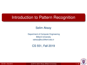
The EM Algorithm in General: the E-stepIE-step maximizes L(q, θ) w.r.t. q for fixed θL(q, θ) ln p(X θ) KL(q(Z)kp(Z X, θ))IL maximized for q(Z) p(Z X, θ)KL(q p) 0KL(q p)L(q, θ)ln p(X θ)Thomas Mensink, Jakob VerbeekL(q, θ old )ln p(X θ old )Bishop Chapter 9: Mixture Models and EM

The EM Algorithm in General: the M-stepIM-step maximizes L(q, θ) w.r.t. θ for fixed qXXL(q, θ) q(Z) ln p(X, Z θ) q(Z) ln q(Z)ZIZL maximized for θ arg maxθPZ q(Z) ln p(X, Z θ)KL(q p)KL(q p) 0KL(q p)L(q, θ)ln p(X θ)L(q, θ old )Thomas Mensink, Jakob Verbeekln p(X θ old )L(q, θ new )ln p(X θ new )Bishop Chapter 9: Mixture Models and EM

The EM Algorithm in General: picture in parameter spaceIE-step resets bound L(q, θ) on ln p(X θ) at θ θold , it isIIItight at θ θoldtangential at θ θoldconvex (easy) in θ for exponential family mixture components Thomas Mensink, Jakob VerbeekBishop Chapter 9: Mixture Models and EM

The EM Algorithm in General: Final ThoughtsI(local) maxima of L(q, θ) correspond to those of ln p(X θ)IEM converges to (local) maximum of likelihoodIICoordinate ascent on L(q, θ), and L ln p(X θ) after E-stepAlternative schemes to optimize the boundIIIIGeneralized EM: relax M-step from maxmizing to increasing LExpectation Conditional Maximization: M-step maximizesw.r.t. groups of parameters in turnIncremental EM: E-step per data point, incremental M-stepVariational EM: relax E-step from maximizing to increasing LIIno longer L ln p(X θ) after E-stepSame applies for MAP estimation p(θ X) p(θ)p(X θ)/p(X)Ibound second term: ln p(θ X) ln p(θ) L(q, θ) ln p(X)Thomas Mensink, Jakob VerbeekBishop Chapter 9: Mixture Models and EM

An Alternative View of EM: latent variables I Let X observed data, Z latent variables, θ parameters. I Goal: maximize marginal log-likelihood of observed data lnp(X θ) ln (X Z p(X,Z θ)). (9.29) I Optimization problematic due to log-sum. I Assume straightforward maximization for complete data lnp(X,Z θ). I Latent Z is known only through p(Z X,θ). I We will consider expectation of .