WIXLIB

GEOPHYSICAL RESEARCH LETTERS, VOL. , NO. , PAGES 1–12,Measuring the Sea Breeze from QuikSCAT ScatterometrySarah T. GilleScripps Institution of Oceanography and Department of Mechanical and Aerospace Engineering, University of California,San DiegoStefan G. Llewellyn SmithDepartment of Mechanical and Aerospace Engineering, University of California, San DiegoShira M. LeeMassachusetts Institute of TechnologyAbstract. Differences between morning and evening winds fromQuikSCAT scatterometer measurements are analyzed to diagnosethe diurnal variability of the wind over the ocean. A statisticallysignificant signal, associated with the sea breeze, is present alongmost of the world’s coastlines. Significant diurnal variability is alsopresent mid-ocean in the easterly trade wind belts.1. IntroductionSea breezes are caused by differential heating of the land andocean. As the land warms during the day, denser air from theadjacent ocean flows over the land. At night, the flow pattern reverses. Simpson [1994] provides a comprehensive overview of thesea breeze, which has implications for coastal physical oceanography, coastal meteorology, and atmospheric pollution.The structure of the sea breeze over land has been observedfor more than a century using land-based meteorological stations[e.g. Davis et al., 1890]. In past studies aircraft measurements,regional radar, and meteorological buoys have been used to probethe offshore structure of the sea breeze [e.g. Atkins et al., 1995].These studies have elucidated the characteristics of the sea breezeonly in areas where field observations have been conducted. Forexample, along the Baltic coast the landward and seaward reach ofthe sea breeze are about the same, with effects felt approximately50 km inland and out to sea [Rossi, 1957; Simpson, 1994]. Similarestimates on a global scale have not been possible to date.Satellite scatterometry now allows us to obtain measurementsof wind speed and direction globally, including along ice-freecoastlines. This study uses vector wind fields obtained from theQuikSCAT satellite scatterometer to examine the amplitude, direction, and offshore extent of the sea breeze.2. Scatterometer DataThe QuikSCAT satellite was launched in July 1999. Its SeaWinds scatterometer measures backscattered microwave power,which is translated into 10-m wind speed and direction along an1800 km wide swath. The satellite orbit is optimized to measurewinds over 90% of the Earth at least once per day. QuikSCATCopyright by the American Geophysical Union.Paper number .0094-8276/02/ 5.001

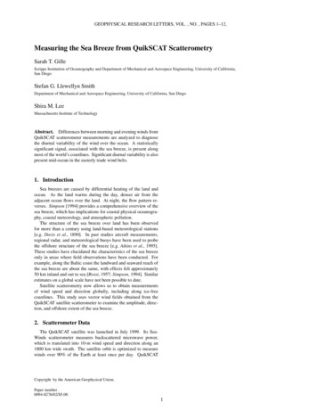
2GILLE ET AL.: SEA BREEZE FROM SCATTEROMETRYfollows a sun-synchronous orbit: the nadir beam, directly belowthe satellite, measures winds around 6:00 local time for ascending satellite passes and around 18:00 local time for descendingsatellite passes [Longu, 2001]. Figure 1 shows the time range ofmeasurements as a function of latitude. Compared to the 3- to6-hourly Comprehensive Ocean-Atmosphere Data Set used by Daiand Deser [1999] to study diurnal variations in global surface winds,QuikSCAT offers coarser temporal sampling but higher spatial resolution. The major focus of this paper is the coastal sea breeze,which requires high spatial resolution sampling.Gridded products have been developed based on QuikSCATwinds. However, we work with swath winds to retain the original spatial resolution and temporal sampling information in thedata. The winds are initially processed by Remote Sensing Systems(www.remss.com). We use compact level 2B data files produced byFlorida State University’s Center for Ocean-Atmosphere PredictionStudies. The data in this analysis span a 3 year period from 31 July1999 to 30 July 2002. Swath winds are reported in 25 km by 25 kmpixels. The pixels have different coordinates each day, dependingon the exact location of the satellite. For this analysis, we averagedeastward (u) and northward (v) components of the morning andevening data into 0.4 latitude by 0.4 longitude bins for the globalocean. Results based on 0.2 boxes are consistent with the resultsreported here.3. Analysis of the Sea BreezeFigure 2a shows for the global ocean the amplitude and directionof the mean wind ū 12 (uam upm ), representing the averageof morning and evening passes, where u (u, v) is the vectorwind. For each box the error of the wind components u and v wasestimated for both morning and evening winds by computing twicethe standard deviation of u and v divided by the square root of thenumber of samples. The error of the mean is then half the squareroot of the sum of these four error components squared. Whiteregions in Figure 2a indicate places where the mean wind is notstatistically different from zero.Because the sea breeze is characterized by a reversal of thewind on a daily basis, we computed the difference between themorning and evening satellite passes to identify the sea breeze.Figure 2b shows the amplitude and direction of the difference u uam upm . The error in u is twice the error in ū. Speeds anddirections have been plotted only if the difference between morningand evening passes is statistically different from zero.Statistically significant values of u occur along most of thecoastlines of the world. However, the most visible feature in Figure 2b is the large band of small but statistically significant u inthe trade wind belt, between 30 S and 30 N. The open-ocean vectors in Figure 2b indicate that flow is more poleward in the morningand more equatorward in the evening, implying a divergence of thewind in the morning and a convergence in the evening, most likelylinked to enhanced daytime rising air motions in the tropics relativeto the subtropics. This is consistent with Dai and Deser [1999],who reported a maximum in surface wind divergence around 6:00in much of the tropical Pacific. The zonal bands of white in between about 5 N and 10 N in Figure 2b appear to coincide with theIntertropical Convergence Zone.The easterly trade winds in Figure 2a average between 5 and10 m s 1 , so the diurnal cycle in Figure 2b represents a smallperturbation to this mean flow. For comparison, in Figure 2c,the amplitude and direction of u is plotted only in locationswhere it exceeds the component of mean flow in the same direction,i.e. u 2 u · ū , so that the wind reverses direction between

GILLE ET AL.: SEA BREEZE FROM SCATTEROMETRYmorning and evening. This flow reversal occurs primarily alongcoastlines, with directional vectors in Figure 2c indicating that thewinds are offshore in the morning and onshore in the evening.This reversal can be thought of as a signature of the sea breeze.Significant sea breezes are found along most of the coastlines of theworld, including for example, along the western Mediterranean Sea,along the west coast of Africa, and around most of the islands of theIndonesian Archipelago. The sea breeze speeds plotted in Figure 2care strongest at points closest to the coast and decrease with distanceoffshore. However, along the west coast of South America and thesouthwest coast of Africa, the sea breeze appears displaced fromthe coast. Poleward of 50 , the sea breeze is noticeably diminished,and in many places no diurnal difference is observed. The lack ofsea breeze signal at high latitudes is not an artifact of the temporalsampling: narrowing the morning and evening time window to 3hours in order to ensure that high-latitude measurements were fromthe same time of day had little impact on the results.The sea breeze is generated by solar heating of the land, and thecorresponding sea-breeze front propagates onshore as a gravity current. Because of the twice-daily sampling provided by QuikSCAT,we cannot see this propagation. In an analysis of buoy data offthe coast of southern California, Lerczak et al. [2001] found thatmaximum onshore winds on the shoreline were 2.7 hours after localnoon, while 220 km offshore, the maximum onshore winds occurred9 hours after local noon. Since QuikSCAT measures six hours afterlocal noon, we expect to sample the maximum amplitude of thediurnal cycle at a location several hundred kilometers offshore. IfQuikSCAT observations were collected closer to noon, we mightexpect to see a more pronounced sea breeze in coastal bins, and thewhite areas off the west coasts of South America and Africa mightnot extend all the way to the coast.Sea breezes are predicted to rotate anticyclonically through thecourse of the day [e.g. Haurwitz, 1947]. Depending on the timingof solar forcing effects compared with the QuikSCAT samplingtime, the sea breeze could be observed with a variety of differentorientations relative to the coastline. The temporal and spatialsampling of the scatterometer did not allow us to investigate therotation in detail. Lerczak et al. [2001] showed that the major axisof wind variability on the beach in San Diego is offset between 30 and 45 from the axis of the coastline. In contrast, at locationsbetween 60 and 220 km offshore, the major axis of wind variabilitywas perpendicular to the coast. The results in Figure 2b,c areconsistent with Lerczak et al.’s [2001] findings, showing that in thelocations resolved by QuikSCAT, which are generally at least 30 kmfrom the shore, the sea breeze is perpendicular to the coastline.4. Offshore Extent of the Sea BreezeThe offshore extent of the sea breeze varies with location: itis about 200 km off the west coast of the Sahara Desert in Africa,400 km south of Australia, and extends northward from the YucatánPeninsula across almost the entire Gulf of Mexico. Using lineartheory, Niino [1987] argued that the offshore extent of the seabreeze should vary by about a factor of 3 as a function of latitude,with the sea breeze extending further out to sea in lower latitudes,as is observed here. Numerical simulations have also found thistrend [Yan and Anthes, 1987; Ciesielski et al., 2001].In most locations the sea breeze extends out to sea from thecoast, but off the west coasts of South America and Africa, asnoted above, it does not. Both locations are in the trade-wind beltand are distinguished by high mountains not far from the coastline.Adjacent to the Andes, in particular, mean winds (Figure 2a) and thedaily cycle (Figure 2b) both flow parallel to the coast, probably as3