Transcription
V. Kumar5. Introduction to Robot Geometry and KinematicsThe goal of this chapter is to introduce the basic terminology and notation used in robot geometryand kinematics, and to discuss the methods used for the analysis and control of robotmanipulators. The scope of this discussion will be limited, for the most part, to robots withplanar geometry. The analysis of manipulators with three-dimensional geometry can be found inany robotics text1.5.1 Some definitions and examplesWe will use the term mechanical system to describe a system or a collection of rigid or flexiblebodies that may be connected together by joints. A mechanism is a mechanical system that hasthe main purpose of transferring motion and/or forces from one or more sources to one or moreoutputs. A linkage is a mechanical system consisting of rigid bodies called links that areconnected by either pin joints or sliding joints. In this section, we will consider mechanicalsystems consisting of rigid bodies, but we will also consider other types of joints.Degrees of freedom of a systemThe number of independent variables (or coordinates) required to completely specifythe configuration of the mechanical system.While the above definition of the number of degrees of freedom is motivated by the need todescribe or analyze a mechanical system, it also is very important for controlling or driving amechanical system. It is also the number of independent inputs required to drive all the rigidbodies in the mechanical system.Examples:(a) A point on a plane has two degrees of freedom. A point in space has three degrees offreedom.(b) A pendulum restricted to swing in a plane has one degree of freedom.1Inparticular, two books offer an excellent treatment while keeping the mathematics at a very simple level: (a) Craig,J. J. Introduction to Robotics, Addison-Wesley, 1989; and (b) Paul, R., Robot Manipulators, Mathematics,Programming and Control, The MIT Press, Cambridge, 1981.-1-
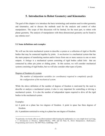
(c) A planar rigid body (or a lamina) has three degrees of freedom. There are two if you considertranslations and an additional one when you include rotations.(d) The mechanical system consisting of two planar rigid bodies connected by a pin joint hasfour degrees of freedom. Specifying the position and orientation of the first rigid bodyrequires three variables. Since the second one rotates relative to the first one, we need anadditional variable to describe its motion. Thus, the total number of independent variables orthe number of degrees of freedom is four.(e) A rigid body in three dimensions has six degrees of freedom. There are three translatorydegrees of freedom. In addition, there are three different ways you can rotate a rigid body.For example, consider rotations about the x, y, and z axes. It turns out that any rigid bodyrotation can be accomplished by successive rotations about the x, y, and z axes. If the threeangles of rotation are considered to be the variables that describe the rotation of the rigidbody, it is evident there are three rotational degrees of freedom.(f) Two rigid bodies in three dimensions connected by a pin joint have seven degrees offreedom. Specifying the position and orientation of the first rigid body requires six variables.Since the second one rotates relative to the first one, we need an additional variable todescribe its motion. Thus, the total number of independent variables or the number of degreesof freedom is seven.Kinematic chainA system of rigid bodies connected together by joints. A chain is called closed if itforms a closed loop. A chain that is not closed is called an open chain.Serial chainIf each link of an open chain except the first and the last link is connected to two otherlinks it is called a serial chain.An example of a serial chain can be seen in the schematic of the PUMA 560 series robot2, anindustrial robot manufactured by Unimation Inc., shown in Figure 1. The trunk is bolted to afixed table or the floor. The shoulder rotates about a vertical axis with respect to the trunk. Theupper arm rotates about a horizontal axis with respect to the shoulder. This rotation is theshoulder joint rotation. The forearm rotates about a horizontal axis (the elbow) with respect tothe upper arm. Finally, the wrist consists of an assembly of three rigid bodies with three2TheProgrammable Universal Machine for Assembly (PUMA) was developed in 1978 by Unimation Inc. using a setof specifications provided by General Motors.Robot Geometry and Kinematics-2-V. Kumar
additional rotations. Thus the robot arm consists of seven rigid bodies (the first one is fixed) andsix joints connecting the rigid bodies.Figure 1 The six degree-of-freedom PUMA 560 robot manipulator.Figure 2 The six degree-of-freedom T3 robot manipulator.Robot Geometry and Kinematics-3-V. Kumar
Another schematic of an industrial robot arm, the T3 made by Cincinnati Milacron, is shownin Figure 2. Once again, it is possible to model it as a collection of seven rigid bodies (the firstbeing fixed) connected by six joints3.Types of jointsThere are mainly four types of joints that are found in robot manipulators: Revolute, rotary or pin joint (R) Prismatic or sliding joint (P) Spherical or ball joint (S) Helical or screw joint (H)The revolute joint allows a rotation between the two connecting links. The best example of this isthe hinge used to attach a door to the frame. The prismatic joint allows a pure translation betweenthe two connecting links. The connection between a piston and a cylinder in an internalcombustion engine or a compressor is via a prismatic joint. The spherical joint between two linksallows the first link to rotate in all possible ways with respect to the second. The best example ofthis is seen in the human body. The shoulder and hip joints, called ball and socket joints, arespherical joints. The helical joint allows a helical motion between the two connecting bodies. Agood example of this is the relative motion between a bolt and a nut.Planar chainAll the links of a planar chain are constrained to move in or parallel to the same plane.A planar chain can only allow prismatic and revolute joints. In fact, the axes of the revolute jointsmust be perpendicular to the plane of the chain while the axes of the prismatic joints must beparallel to or lie in the plane of the chain.An example of a planar chain is shown in Figure 3. Almost all internal combustion enginesuse a slider crank mechanism. The high pressure of the expanding gases in the combustionchamber is used to translate the piston and the mechanism converts this translatory movementinto the rotary movement of the crank. This mechanical system consists of three revolute jointsand one prismatic joint.The example in Figure 3 is a planar, closed, kinematic chain. Examples of planar, serialchains are shown in Figure 4 and 5.3Thisis a convenient model. A more accurate kinematic model is required to model the coupling between theactuator that drives the elbow joint and the elbow joint.Robot Geometry and Kinematics-4-V. Kumar
Connectivity of a jointThe number of degrees of freedom of a rigid body connected to a fixed rigid bodythrough the joint.The revolute, prismatic and helical joint have a connectivity 1. The spherical joint has aconnectivity of 3. Sometimes one uses the term “degree of freedom of a joint” instead of theconnectivity of a joint.Crank shaftConnectingrodlrτθCylinderφFPistonxFigure 3 A schematic of a slider crank TORSRJointFigure 4 A schematic of a planar manipulator with three revolute jointsRobot Geometry and Kinematics-5-V. Kumar
END-EFFECTORRPACTUATORSRFigure 5 A schematic of a planar manipulator with two revolute and one prismatic jointsMobilityThe mobility of a chain is the number of degrees of freedom of the chain.Most books will use the term “number of degrees of freedom” for the mobility. In a serial chain,the mobility of the chain is easily calculated. If there are n joints and joint i has a connectivity fi,nM fii 1Most industrial robots have either revolute or prismatic joints (fi 1) and therefore the mobilityor the number of degrees of freedom of the robot arm is also equal to the number of joints.Sometimes, an n degree of freedom robot or a robot with mobility n is also called an n axisrobot.Since a rigid body in space has six degrees of freedom, the most general robots are designedto have six joints. This way, the end effector or the link that is furthest away from the base can bemade to assume any position or orientation (within some range). However, if the end effectorneeds to moved around in a plane, the robot need only have three degrees of freedom. Twoexamples4 of planar, three degree of freedom robots (technically, mobility three robots) areshown in Figures 4 and 5.4Notethat we do not count the opening and closing of the gripper as a degree of freedom. The gripper is usuallycompletely open or completely shut and it is not continuously controlled as the other joints are. Also, the gripperfreedom does not participate in the positioning and orienting of a part held by the gripper.Robot Geometry and Kinematics-6-V. Kumar
When closed loops are present in the kinematic chain (that is, the chain is no longer serial, oreven open), it is more difficult to determine the number of degrees of freedom or the mobility ofthe robot. But there is a simple formula that one can derive for this purpose.Let n be the number of moving links and let g be the number of joints, with fi being theconnectivity of joint i. Each rigid body has six degrees if we consider spatial motions. If therewere no joints, since there are n moving rigid bodies, the system would have 6n degrees offreedom. The effect of each joint is to constrain the relative motion of the two connecting bodies.If the joint has a connectivity fi, it imposes (6-fi) constraints on the relative motion. In otherwords, since there are fi different ways for one body to move relative to another, there (6-fi)different ways in which the body is constrained from moving relative to another. Therefore, thenumber of degrees of freedom or the mobility of a chain (including the special case of a serialchain) is given by:gM 6n (6 f i )i 1or,gM 6(n g ) f i(2)i 1END-EFFECTORACTUATORSFigure 6 A planar parallel manipulator.Robot Geometry and Kinematics-7-V. Kumar
In the special case of planar motion, since each unconstrained rigid body has 3 degrees offreedom, this equation is modified to:gM 3(n g ) f i(3)i 1Example 1In Figures 4 and Figure 5, since n g 3, Equation (3) reduces to the special case of Equation(1). And since f1 f2 f3 1, and M g.Example 2In the slider crank mechanism shown in Figure 3, n 3 andg 4. Since it is a planar mechanismwe use Equation (2). All four joints have connectivity one: f1 f2 f3 f4 1, and M 1.Example 3Consider the parallel manipulator shown in Figure 6. Here, n 7, g 9, and fi 1. According toEquation (3), M 3. There are correspondingly three actuators in the manipulator. Contrastthis arrangement with the arrangement shown in Figures 4 and 5. The three actuators aremounted in parallel in Figure 6. In Figures 4 and 5, they are mounted “sequentially” in aserial fashion.The Stewart PlatformThe Stewart-Gough or the Stewart Platform5 device is a six degree of freedom (mobility six)kinematic chain with closed loops. The kinematic chain consists of a base and a moving platformeach of which is a spatial hexagon. See Figure 7. Every vertex of the base hexagon is connectedto one vertex of the moving platform hexagon by one leg. Similarly, every vertex of the movinghexagon is connected to a vertex of the base hexagon by a leg. There are six such legs. Each leghas is a serial chain consisting of two revolute joints with intersecting axes, a prismatic joint anda spherical joint. Typically the prismatic joints are actuated.The mobility of a Stewart Platform can be easily verified to be six. Each leg has three linksand four joints. If we include the moving platform,n 6 3 1 19.5D.Stewart, “A Platform with Six Degrees of Freedom,” The Institution of Mechanical Engineers, Proceedings1965-66, Vol. 180 Part 1, No. 15, pages 371-386.Robot Geometry and Kinematics-8-V. Kumar
(a) A machine tool based on the Stewart Platform (Ingersoll Rand)6SEND EFFECTORPLeg 5Leg 4Leg 6RLeg 3Leg 2Leg 1RBASELEG NO. i(b) A schematic showing the six legs (left) and the RRPS chain (right).Figure 76M.The Stewart PlatformValenti, “Machine Tools Get Smarter,” Mechanical Engineering, Vol.117, No.11, November 1995.Robot Geometry and Kinematics-9-V. Kumar
The connectivity of the revolute and the prismatic joint is one. The connectivity of the sphericaljoint is three. Since there are 6 2 revolute joints, 6 prismatic joints and 6 spherical joints,g f i 12 6 6 3 36i 1According to Equation (3),M 6(19 24) 36 6The Stewart Platform has actuators for all its six prismatic joints and it is therefore possible tocontrol all six degrees of freedom.(a) The Adept 1850 Palletizer(b) side view (axes 2-4 are numbered)(c) top view (axes 2-4 are numbered)Figure 8 The Adept 1850 PalletizerThere are four degrees of freedom in this SCARA manipulator. Joint 1 is a slidingjoint that carries the manipulator arm up or down. Joints 2-4 are rotary joints withvertical axes.Robot Geometry and Kinematics-10-V. Kumar
5.2 Geometry of planar robot manipulatorsThe mathematical modeling of spatial linkages is quite involved. It is useful to start withplanar robots because the kinematics of planar mechanisms is generally much simpler to analyze.Also, planar examples illustrate the basic problems encountered in robot design, analysis andcontrol without having to get too deeply involved in the mathematics. However, while theexamples we will discuss will involve kinematic chains that are planar, all the definitions andideas presented in this section are general and extend to the most general spatial mechanisms.We will start with the example of the planar manipulator with three revolute joints. Themanipulator is called a planar 3R manipulator. While there may not be any three degree offreedom (d.o.f.) industrial robots with this geometry, the planar 3R geometry can be found inmany robot manipulators. For example, the shoulder swivel, elbow extension, and pitch of theCincinnati Milacron T3 robot (Figure 2) can be described as a planar 3R chain. Similarly, in afour d.o.f. SCARA manipulator (Figure 8), if we ignore the prismatic joint for lowering or raisingthe gripper, the other three joints form a planar 3R chain. Thus, it is instructive to study theplanar 3R manipulator as an example.In order to specify the geometry of the planar 3R robot, we require three parameters, l1, l2,and l3. These are the three link lengths. In Figure 9, the three joint angles are labeled θ1, θ2, andθ3. These are obviously variable. The precise definitions for the link lengths and joint angles areas follows. For each pair of adjacent axes we can define a common normal or the perpendicularbetween the axes. The ith common normal is the perpendicular between the axes for joint i and joint i 1. The ith link length is the length of the ith common normal, or the distance between the axesfor joint i and joint i 1. The ith joint angle is the angle between the (i-1)th common normal and ith commonnormal measured counter clockwise going from the (i-1)th common normal to the ithcommon normal.Note that there is some ambiguity as far as the link length of the most distal link and the jointangle of the most proximal link are concerned. We define the link length of the most distal linkfrom the most distal joint axis to a reference point or a tool point on the end effector7. Generally,this is the center of the gripper or the end point of the tool. Since there is no zeroth commonnormal, we measure the first joint angle from a convenient reference line. Here, we have chosenthis to be the x axis of a conveniently defined fixed coordinate system.7Thereference point is often called the tool center point (TCP).Robot Geometry and Kinematics-11-V. Kumar
Another set of variables that is useful to define is the set of coordinates for the end effector.These coordinates define the position and orientation of the end effector. With a convenientchoice of a reference point on the end effector, we can describe the position of the end effectorusing the coordinates of the reference point (x, y) and the orientation using the angle φ. The threeend effector coordinates (x, y, φ) completely specify the position and orientation of the endeffector8.REFERENCEPOINTφ(x, y)l3θ3l2yθ2l1θ1xFigure 9 The joint variables and link lengths for a 3R planar manipulatorAs another example, consider the three d.o.f. cylindrical robot in Figure 10. If we ignore thelift freedom, the rotation of the base and the extension of the arm give us the two d.o.f. robotshown in Figure 11 that we can call the R-P manipulator. It consists of a revolute joint andprismatic joint as shown in the figure. θ1, the base rotation, and d2, the arm extension, are the twojoint variables. Note that there are no constant parameters such as the three link lengths in the 3Rmanipulator. The joint variable θ1 is defined as before. Since there is no zeroth common normal,8Thedescription of the position and orientation of a three dimensional rigid body is significantly more complicated.For a spatial manipulator, a typical set of end effector coordinates would include three variables (x, y, z) for theposition, and three Euler angles (θ, φ, ψ) for the orientation.Robot Geometry and Kinematics-12-V. Kumar
we measure the joint angle from the x axis which we have chosen to be horizontal. d2 is definedas the distance from joint axis 1 to the reference point on the end effector. As in the previousexample, the end effector coordinates are variables that completely specify the position andorientation of the end effector. In the figure, they are (x, y, φ).Finally, we consider a Cartesian robot consisting of two prismatic joints at right angles. TheP-P chain is found in x-y tables, plotters and milling machines. A schematic is shown in Figure12. The simplest spatial manipulator is based on the P-P-P chain, which has a third prismaticjoint. The three joint axes are mutually orthogonal. The Gantry robot in Figure 13 has thisgeometry. If you ignore the vertical up/down degree of freedom it is a P-P manipulator.Figure 10 The RT3300 cylindrical robot (Seiko)REFERENCEPOINT(x, y)d2y2θ11φxFigure 11 The joint variables and link lengths for a R-P planar manipulatorRobot Geometry and Kinematics-13-V. Kumar
d2d1Figure 12 The joint variables for a P-P planar manipulatorFigure 13 The G365 Gantry robot manipulator (CRS Robotics) on the left, and the Biomek2000 Laboratory Automation Workstation (Beckman Coulter) on the right both have toolingmounted at the end of a P-P-P chain.The end effector of a manipulator that has only prismatic joints is constrained to remain inthe same orientation. Thus, the end effector coordinates for the P-P manipulator only include thecoordinates of the reference point on the end effector (x, y).In summary, in each case, we defined a set of constant parameters called link lengths (li) andset of joint variables or joint coordinates consisting of either joint angles (θi) or displacementsRobot Geometry and Kinematics-14-V. Kumar
(di). We also defined a set of variables called end effector coordinates. The link lengths areconstant parameters that define the geometry of the manipulator. The joint variables define theconfiguration of the manipulator by specifying the position of each joint. The end effectorcoordinates define the position and orientation of the end effector. If the joint coordinates specifythe configuration of the manipulator, they should also specify the position and orientation of theend effector. Thus one should expect to find an explicit dependence of the end effectorcoordinates on the joint coordinates. Although it may not be obvious, there is also a dependenceof the joint coordinates on the end effector coordinates. The next subsection will address thisdependence and analyse the kinematics of robot manipulators.5.3 Kinematic analysis of planar serial chainsKinematics is the study of motion. In this subsection, we will explore the relationshipbetween joint movements and end effector movements. More precisely, we will try to developequations that will make explicit the dependence of end effector coordinates on joint coordinatesand vice versa.We will start with the example of the planar 3R manipulator. From basic trigonometry, theposition and orientation of the end effector can be written in terms of the joint coordinates in thefollowing way:x l1 cos θ1 l2 cos(θ1 θ2 ) l3 cos(θ1 θ2 θ3 )y l1 sin θ1 l2 sin (θ1 θ2 ) l3 sin (θ1 θ2 θ3 )(4)φ (θ1 θ2 θ3 )Note that all the angles have been measured counter clockwise and the link lengths are assumedto be positive going from one joint axis to the immediately distal joint axis.Equation (4) is a set of three nonlinear equations9 that describe the relationship between endeffector coordinates and joint coordinates. Notice that we have explicit equations for the endeffector coordinates in terms of joint coordinates. However, to find the joint coordinates for agiven set of end effector coordinates (x, y, φ), one needs to solve the nonlinear equations for θ1,θ2, and θ3.The kinematics of the planar R-P manipulator is easier to formulate. The equations are:9Thethird equation is linear but the system of equations is nonlinear.Robot Geometry and Kinematics-15-V. Kumar
x d 2 cos θ1y d 2 sin θ1(5)φ θ1Again the end effector coordinates are explicitly given in terms of the joint coordinates.However, since the equations are simpler (than in (4)), you would expect the algebra involved insolving for the joint coordinates in terms of the end effector coordinates to be easier. Notice thatin contrast to (4), now there are three equations in only two joint coordinates, θ1, and d2. Thus, ingeneral, we cannot solve for the joint coordinates for an arbitrary set of end effector coordinates.Said another way, the robot cannot, by moving its two joints, reach an arbitrary end effectorposition and orientation.Let us instead consider only the position of the end effector described by (x, y), thecoordinates of the end effector tool point or reference point . We have only two equations:x d 2 cos θ1(6)y d 2 sin θ1Given the end effector coordinates (x, y), the joint variables can be computed to be:d2 x2 y2(7) y θ1 tan 1 x Notice that we restricted d2 to positive values. A negative d2 may be physically achieved byallowing the end effector reference point to pass through the origin of the x-y coordinate systemover to another quadrant. In this case, we obtain another solution:d2 x2 y2(8) y θ1 tan 1 x In both cases (7-8), the inverse tangent function is multivalued10. In particular,(9)tan(x) tan(x kπ), k -2, -1, 0, 1, 2, However, if we limit θ1 to the range 0 θ1 2π, there is a unique value of θ1 that is consistent withthe given (x, y) and the computed d2 (for which there are two choices).10InAppendix 1, we define another inverse tangent function called atan2 that takes two arguments, the sine and thecosine of an angle, and returns a unique angle in the range [0, 2π).Robot Geometry and Kinematics-16-V. Kumar
The existence of multiple solutions is typical when we solve nonlinear equations. As we willsee later, this poses some interesting questions when we consider the control of robotmanipulators.The planar Cartesian manipulator is trivial to analyze. The equations for kinematic analysisare:x d2,y d1(10)The simplicity of the kinematic equations makes the conversion from joint to end effectorcoordinates and back trivial. This is the reason why P-P chains are so popular in suchautomation equipment as robots, overhead cranes, and milling machines.Direct kinematicsAs seen earlier, there are two types of coordinates that are useful for describing theconfiguration of the system. If we focus our attention on the task and the end effector, we wouldprefer to use Cartesian coordinates or end effector coordinates. The set of all such coordinates isgenerally referred to as the Cartesian space or end effector space11. The other set of coordinatesis the so called joint coordinates that is useful for describing the configuration of the mechanicallnkage. The set of all such coordinates is generally called the joint space.In robotics, it is often necessary to be able to “map” joint coordinates to end effectorcoordinates. This map or the procedure used to obtain end effector coordinates from jointcoordinates is called direct kinematics.For example, for the 3-R manipulator, the procedure reduces to simply substituting the valuesfor the joint angles in the equationsx l1 cos θ1 l2 cos(θ1 θ2 ) l3 cos(θ1 θ2 θ3 )y l1 sin θ1 l2 sin (θ1 θ2 ) l3 sin (θ1 θ2 θ3 )φ (θ1 θ2 θ3 )and determining the Cartesian coordinates, x, y, and φ. For the other examples of open chainsdiscussed so far (R-P, P-P) the process is even simpler (since the equations are simpler). In fact,for all serial chains (spatial chains included), the direct kinematics procedure is fairly straightforward.On the other hand, the same procedure becomes more complicated if the mechanism containsone or more closed loops. In addition, the direct kinematics may yield more than one solution or11Sinceeach member of this set is an n-tuple, we can think of it as a vector and the space is really a vector space. Butwe shall not need this abstraction here.Robot Geometry and Kinematics-17-V. Kumar
no solution in such cases. For example, in the planar parallel manipulator in Figure 3, the jointpositions or coordinates are the lengths of the three telescoping links (q1, q2, q3) and the endeffector coordinates (x, y, φ) are the position and orientation of the floating triangle. It can beshown that depending on the value of (q1, q2, q3), the number of (real) solutions for (x, y, φ) canbe anywhere from zero to six. For the Stewart Platform in Figure 4, this number has been shownto be anywhere from zero to forty.5.4 Inverse kinematicsThe analysis or procedure that is used to compute the joint coordinates for a given set of endeffector coordinates is called inverse kinematics. Basically, this procedure involves solving a setof equations. However the equations are, in general, nonlinear and complex, and therefore, theinverse kinematics analysis can become quite involved. Also, as mentioned earlier, even if it ispossible to solve the nonlinear equations, uniqueness is not guaranteed. There may not (and ingeneral, will not) be a unique12 set of joint coordinates for the given end effector coordinates.We saw that for the R-P manipulator, the direct kinematics equations are:x d 2 cos θ1(6)y d 2 sin θ1If we restrict the revolute joint to have a joint angle in the interval [0, 2π), there are two solutionsfor the inverse kinematics: y x d 2 σ x 2 y 2 , θ1 atan 2 , , σ 1 d2 d2 Here we have used the atan2 function in Appendix 1 to uniquely specify the joint angle θ1.However, depending on the choice of σ, there are two solutions for d2, and therefore for θ1.The inverse kinematics analysis for a planar 3-R manipulator appears to be complicated butwe can derive analytical solutions. Recall that the direct kinematics equations (4) are:x l1 cos θ1 l 2 cos(θ1 θ 2 ) l3 cos(θ1 θ 2 θ 3 )y l1 sin θ1 l 2 sin (θ1 θ 2 ) l3 sin (θ1 θ 2 θ 3 )φ (θ1 θ 2 θ 3 )(4a)(4b)(4c)12Theonly case in which the analysis is trivial is the P-P manipulator. In this case, there is a unique solution for theinverse kinematics.Robot Geometry and Kinematics-18-V. Kumar
We assume that we are given the Cartesian coordinates, x, y, and φ and we want to find analyticalexpressions for the joint angles θ1, θ2, and θ3 in terms of the Cartesian coordinates.Substituting (4c) into (4a) and (4b) we can eliminate θ3 so that we have two equations in θ1and θ2:x l3 cos φ l1 cos θ1 l 2 cos(θ1 θ 2 )y l3 sin φ l1 sin θ1 l2 sin (θ1 θ2 )(d)(e)where the unknowns have been grouped on the right hand side; the left hand side depends onlyon the end effector or Cartesian coordinates and are therefore known.Rename the left hand sides, x ′ x - l3 cos φ, y ′ y - l3 sin φ, for convenience. We regroupterms in (d) and (e), square both sides in each equation and add them:(x′ l1 cos θ1 )2 (l 2 cos(θ1 θ 2 ))2 ( y ′ l1 sin θ1 )2 (l 2 sin (θ1 θ 2 ))2After rearranging the terms we get a single nonlinear equation in θ1:( 2l1x′) cos θ1 ( 2l1 y′)sin θ1 (x′2 y′2 l12 l22 ) 0(f)Notice that we started with three nonlinear equations in three unknowns in (a-c). We reduced theproblem to solving two nonlinear equations in two unknowns (d-e). And now we have simplifiedit further to solving a single nonlinear equation in one unknown (f).Equation (f) is of the typeP cosα Q sinα R 0(g)Equations of this type can be solved using a simple substitution as shown in Appendix 2. Thereare two solutions for θ1 given by:( x′ 2 y ′ 2 l 2 l 212θ1 γ σ cos 1 222l1 x′ y ′ ) (h)where, x′ y′γ a tan 2 ,22x′ 2 y ′ 2 x′ y ′and , σ 1 .Robot Geometry and Kinematics-19-V. Kumar
Note that there are two solutions for θ1, one corresponding to σ 1, the other corresponding toσ -1. Substituting any one of these solutions back into Equations (d) and (e) gives us:x ′ l1 cos θ1l2y ′ l1 sin θ1sin (θ1 θ 2 ) l2cos(θ1 θ 2 ) This allows us to solve for θ2 using the atan2 function in Appendix 1: y′ l1 sin θ1 x′ l1 cos θ1 θ1θ2 atan 2 ,l2l2 (i)Thus, for each solution for θ1, there is one (unique) solution for θ2.Finally, θ3 can be easily determined from (c):θ3 φ - θ1 - θ2(j)Equations (h-j) are the invers
Robot Geometry and Kinematics -2- V. Kumar (c) A planar rigid body (or a lamina) has three degrees of freedom. There are two if you consider