Transcription
Journal of Applied Mathematics and Physics, 2016, 4, 368-375Published Online February 2016 in SciRes. /10.4236/jamp.2016.42043Exponentially-Fitted 2-Step Simpson’sMethod for Oscillatory/Periodic ProblemsAshiribo Senapon Wusu, Bosede Alfred Olufemi, Akanbi Moses AdebowaleDepartment of Mathematics, Lagos State University, Lagos, NigeriaReceived 15 December 2015; accepted 23 February 2016; published 26 February 2016Copyright 2016 by authors and Scientific Research Publishing Inc.This work is licensed under the Creative Commons Attribution International License (CC tractFollowing a six-step flow chart, exponentially-fitted variant of the 2-step Simpson’s method suitable for solving ordinary differential equations with periodic/oscillatory behaviour is constructed.The qualitative properties of the constructed methods are also investigated. Numerical experiments on standard problems confirming the theoretical expectations regarding the constructedmethods compared with other existing standard methods are also presented. Our results unifyand improve the existing classical 2-step Simpson’s method.KeywordsExponentially-Fitted, Simpson Method, Oscillatory, Periodic, ODE1. IntroductionIn this paper, we consider the first-order initial value problem of the formη0u′ f ( t , u ) , t [ t0 , T ] , u ( t0 ) (1)with oscillatory/periodic solution.Several classical methods ([1]-[5]) for solving (1) have been derived. However, classical methods may not bewell-suited for handling problems with pronounced periodic or oscillatory behaviour, because in order toaccurately achieve this, a very small step size would be required with corresponding decrease in performance,especially in terms of efficiency. To overcome this barrier, classical methods have to be adapted in order toefficiently approach the oscillatory behaviour. The adaptation (which is called “exponential/trigonometricfitting”) is achieved by replacing some of the highest order monomials of the basis with exponentials ortrigonometric (see [6]-[8]). Numerical algorithms for solving problems whose solution exhibits a pronouncedperiodic or oscillatory behaviour has since the last decade gained a lot of attention. Such problems are oftenHow to cite this paper: Wusu, A.S., Olufemi, B.A. and Adebowale, A.M. (2016) Exponentially-Fitted 2-Step Simpson’s Method for Oscillatory/Periodic Problems. Journal of Applied Mathematics and Physics, 4, 368-375.http://dx.doi.org/10.4236/jamp.2016.42043
A. S. Wusu et al.encountered in fields like mechanics, electronic, astrophysics, chemistry and engineering. The idea of usingexponentially fitted formulae for differential equations was first proposed by Liniger and Willoughby [9].Integration formulae containing free parameters were derived and these parameters were chosen so that a givenfunction exp ( q ) where q was real, satisfied the integration formulae exactly. This was tested on linearmultistep method for k 1 , however Jackson and Kenue [10] derived a fourth order exponentially fittedformulae based on a linear 2-step formula and were A-stable. Based on this idea, Cash [11], in his own work,attempted using Multiderivative Linear Multistep Method (MLMM) with k 1 in the second derivativeformulae. Particular Runge-Kutta (RK) algorithms have been proposed by several authors [12]-[15] in order tosolve this class of problems. Vanden Berghe et al. [16] [17] on the other hand, introduced other exponentiallyfitted RK (EFRK) methods which integrate exactly first-order systems whose solutions canbe expressed as linear combinations of functions of the form {exp ( λ t ) , exp ( λ t )} or {cos (ωt ) , sin (ωt )} .Here, we analyze the construction and implementation of the exponentially-fitted variants of the 2-stepSimpson method for solving problems of the form (1) which possess oscillatory/periodic solution, taking intoaccount the six-step flow chart described by Ixaru and Vanden Berghe in [6].The main interest of this work is to modify the classical 2-step Simpson method for adaptation to oscillatory/periodic problems.2. Construction of MethodThe classical 2-step Simpson method for solving (1) is given byun 1 un 1 h( f j 1 4 f j f j 1 ) .3(2)To begin the construction of the exponentially-fitted variants of (2), we rewrite (2) in a more general way asun 1 α 0un 1 h ( β 2 f j 1 β1 f j β 0 f j 1 ) .(3)Following the six-step flow chart, the corresponding linear difference operator [ h, a ] reads [ h, a ] u ( t ) u ( t h ) α 0u ( t h ) h(( β 2u ′ ( t h ) β1u ′ ( t ) β 0u ′ ( t h ) )where a : (α 0 , β 0 , β1 , β 2 )where a : (α 0 , β 0 , β1 , β 2 ) . Applying step II of the six-step procedure, the resulting system of equations iscompatible when M 5 . Solving the resulting system, we have1, β α β 00214, β 133(4)which are the coefficients of the classical method (2).Applying step III, we find that( Z ) (α 1) cosh ( Z ) 1) sinh ( Z ) ( β β ) cosh ( Z )ZG ( Z , a ) ( β 0 β 2 ) Z sinhG ( Z , a) β1 (α 0020(5)(6)z ω h ωh and Z z 2 , ω (the frequency of oscillation) is real or imaginary. (For the trigonometricwhere z ω h i µ h , i.e. z 2 µ 2 h2 Z .)case, i.e., ω is imaginary, choose To implement step IV, consider the reference set of M functions:{1, t , , tK}, exp ( ωt ) , t exp ( ωt ) , , t P exp ( ωt )with K 2 P M 3 . Since for our method M 5 , we have three possibilities: K 4, P 1 , the classical case with the set 1, t , t 2 , t 3 , t 4369
A. S. Wusu et al. K 2, P 0 , the mixed case with the set 1, t , t 2 , exp ( ωt ) K 0, P 1 , the mixed case with the set 1, exp ( ωt ) , t exp ( ωt )The coefficients of the method for each case are obtained by the implementation of step V as follows:S1: ( K , P ) ( 4, 1) In this case, the solution is already known by (4)S2:( K , P ) ( 2, 0 )α 0 1, sinh ( z ) z β2 , z ( cosh ( z ) 1) 2 z csch ( z cosh ( z ) sinh ( z ) ) 2 β1 , z sinh ( z ) z β0 z ( cosh ( z ) 1) S3:(7)( K , P ) ( 0,1)α 0 1, z coth ( z ) 1 ,β2 z2 2 ( cosh ( z ) zcsch ( z ) ) , β1 z2 z coth ( z ) 1β0 2z As expected, the exponentially fitted variants reduce to the the classical method as z 0 .(8)3. Error Analysis: Local Truncation Error (lte)The general expression of the leading term of the local truncation error (lte) for an exponentially fitted methodwith respect to the basis functions{1, t , , tK}, exp ( ωt ) , t exp ( ωt ) , , t P exp ( ωt )(9)takes the form (see [6]) ( a ( Z ) ) K 1 2P 1lte EF ( t ) DD ω2( 1) h M K 1( K 1) ! Z P 1()P 1u (t )(10)with K, P and M satisfying the condition K 2 P M 3 .For the three methods constructed above, one finds the following results: S1: ( K , P ) ( 4, 1)lteEF ( t ) S2:( K , P ) ( 2, 0 )lteEF (t ) S3:1 5 ( 5)h u (t )90(1 535h (α 0 3β 2 3β 0 1) ω 2u ( ) ( t ) u ( ) ( t )6Z(11))( K , P ) ( 0,1)lte EF ( t )(1 553h (α 0 β 2 β1 β 0 1) u ( ) ( t ) 2ω 2u ( ) ( t ) ω 4u ′ ( t )2Z370)
A. S. Wusu et al.4. Existence and Uniqueness of SolutionThe following theorem states conditions of f ( t , u ) which guarantee the existence of a unique solution of theinitial value problem (1)Theorem 1. Let f ( t , u ) be defined and continuous for all points ( t , u ) in the region defined bya t b , u , a and b finite, and let there exist a constant such that, for every t , u , u such that(t, u )and(t, u ) are both in ,()f (t, u ) f t, u u u (12)then if η0 is any given number, there exists a unique solution u ( t ) to the initial value problem (1), whereu ( t ) is continuous and differentiable for all( t , u ) . Lambert [3].The requirement (12) is known as the Lipschitz Condition, and the constant is called the Lipschitzconstant.This condition may be thought of as being intermediate between differentiability and continuity, in the sensethat f ( t , u ) continuously differentiable with respect to u ( t , u ) f ( t , u ) satisfies a Lipschitz Condition w.r.t. u ( t , u ) f ( t , u ) continuous w.r.t. u ( t , u ) In particular, if f ( t , u ) possesses a continuous derivative w.r.t. y for alltheorem()f (t, u ) f t, u f ( t , u )u u u(( t , u ) , then, by the mean value)where u is a point in the interior of the interval whose end-points are u and u , andboth in . Clearly (12) is satisfied if(t, u )and f ( x, u ) u( x ,u ) sup(t, u ) are(13)is chosen.5. Contraction Mapping TheoremIn the sequel, we shall apply the following Contraction Mapping Theorem:Theorem 2. (Contraction Mapping Theorem). Consider a set D n and a function g : D n .Assume D is closed (i.e., it contains all limit points of sequences in D) x D g ( x) D The mapping g is a contraction on D: There exists q 1 such that x, y D : g ( x ) g ( y ) q x yThen( ) there exists a unique x D with g x x for any x( ) D , the fixed point iterates given by x(0 x(k)k 1)( )): g x(ksatisfies the a-priori extimatex ( ) x kqk10x( ) x( )1 qand the a-posteriori error estimate371converges to x as k
A. S. Wusu et al.x ( ) x kqkk 1x( ) x( )1 q6. Application of the Contraction Mapping Theorem to LMMIf h is sufficiently small, implicit LMM methods also have unique solutions given h and u0 , u1 , , uk 1 . To seethis, let be the Lipschitz constant for f. Given ui , , ui k 1 , the value for ui k is obtained by solving theequationui k hβ k f ( ti k , ui k ) gi (14)wherek 1 ( hβ k fi j α j ui j ) ( constant ) gi(15)j 0That is, we are looking for a fixed point of φ ( u ) hβ k f ( ti k , u ) gi(16)If h β k 1 , then φ is a contraction:φ ( u ) φ ( u ) h β k f ( ti k , u ) f ( ti k , u ) h β k u u (17)So by the Contraction Mapping Fixed Point Theorem, φ has a unique fixed point. Any initial guess ui0 kyields a convergent fixed point iteration:(uil k1 hβ k f ti k , uil k)(18)7. Convergence and Stability AnalysisTheorem 3 (Dahlquist Theorem) The necessary and sufficient conditions for a linear multistep method to beconvergent are that it be consistent and zero-stableDahlquist theorem (3) holds also true for EF-based algorithms but, because their coefficients are no longerconstants the concepts of consistency and stability have to be adapted.Definition 4. An exponentially fitted method associated with the fitting space (9) is said to be of order p M r , (where r is the order of the differential equation to be solved) and it is consistent if p 1 .Since M 1 for all the constructed schemes, the consistency requirement is satisfied. Hence, the constructedschemes are all consistent.Definition 5. A linear s-step method is said to be weakly stable if there is more than one simple root of thepolynomial equation ρ (ξ ) 0 on the unit circle.To investigate the stability of (3), one applies the method to the test problems u ′ λ u . Applying (3) to theabove test problems, one obtainsun 1 α 0un 1 h ( β 2 λ un 1 β1λ un β 0 λ un 1 ) α 0un 1 λ h ( β 2un 1 β1un β 0un 1 )(19)From the above, one finds that(1 β h ) u2n 1 β1hun (α 0 β 0 h ) un 1 0, n 1, 2, (20)where h λ h . The characteristics equation is given by(1 β h ) ξ22 β1h ξ (α 0 β 0 h ) 0(21)0 . The roots are ξ 1 andsetting h 0 in (21), gives the reduced characteristic equation as ξ 2 1 hence the methods derived are weakly stable. Notice that h depends on the test equation but Z on thenumerical method.372
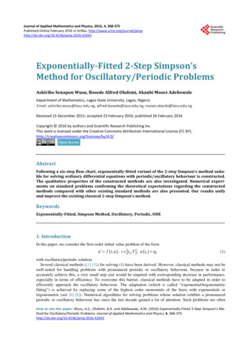
A. S. Wusu et al.Definition 6. A region of stability is a region of the q--z plane, throughout which R ( q, z ) 1 . Any closedcurve defined by R ( q, z ) 1 is a stability boundary. Also, any interval (α , β ) of the real line is said to bethe interval of stability if the method is stable for all q (α , β )For each of the constructed methods, the region of stability is presented in Figure 1.8. Numerical ResultsNumerical experiments confirming the theoretical expectations regarding the constructed methods are nowperformed. The constructed methods are applied to two test problems and the result obtained compared with theclassical fourth-order Taylor method, explicit four stage fourth-order Runge-Kutta method and the classical2-step Simpson method.8.1. Problem 1 u t , u Consider the IVP: u ′ ( 0 ) 1 with the exact solution u ( t ) 2et t 1 . Solving the problem usingdifferent values of steplength h, the the maximum absolute errors for each steplength is obtained as presented inFigure 2. As expected, the exponentially-fitted variants (S2:(2,0), S3:(0,1)) of the classical 2-step Simpsonmethod performed better compared with the classical methods.8.2. Problem 2Consider the IVP: u ′ α u eα t t , u ( 1) e α with the exact solution u ( t ) teα t . With α 1 , the problemis solved using different values of steplength h and the maximum absolute error for each steplength is obtainedas presented in Figure 3. The constructed exponentially fitted variants also performed better compared to theclassical methods.Figure 1. Truncated absolute stability regions of the constructed methods. kh 2 , k 2 (1) 8 . Figure 2. Maximum absolute errors for Problem 1 as a function of the step-size373
A. S. Wusu et al. k h 2 , k 2 (1) 8 , α 1 .Figure 3. Maximum absolute errors for Problem 1 as a function of the step-size9. ConclusionThe exponentially-fitted versions of the classical 2-step Simpson method have been constructed and implemented in this paper. The stability and convergence properties of the constructed methods were also analysed.The results obtained from the numerical examples show that the theoretical expectations are meet (i.e. the exponentially-fitted variants of the classical 2-step Simpson method are suitable for solving periodic/oscillatoryproblems).AcknowledgementsWe thank the Editor and the referee for their comments.References[1]Akan
Simpson method for solving problems of the form (1) which possess oscillatory/periodic solution, taking into account the six-step flow chart described by Ixaru and Vanden Berghe in [6]. The main interest of this work is to modify the classical 2-step Simpson method for adaptation to oscillatory/ periodic problems. 2. Construction of Method