Transcription
CHAPTER 9 ANALYSIS EXAMPLES REPLICATION SPSS/PASW V18GENERALIZED LINEAR MODELS FOR MULTINOMIAL, ORDINAL AND COUNT VARIABLESGENERAL NOTES ABOUT ANALYSIS EXAMPLES REPLICATIONThese examples are intended to provide guidance on how to use the commands/procedures for analysis of complex sample survey data and assume all datamanagement and other preliminary work is done. The relevant syntax for the procedure of interest is shown first along with the associated output forthat procedure(s). In some examples, there may be more than one block of syntax and in this case all syntax is first presented followed by theoutput produced.In some software packages certain procedures or options are not available but we have made every attempt to demonstrate how to match the outputproduced by Stata 10 in the textbook. Check the ASDA website for updates to the various software tools we cover.NOTES ABOUT GENERALIZED LINEAR MODELS IN SPSS/PASW V18 COMPLEX SAMPLES MODULESPSS/PASW ORDINAL commands can perform some of the analyses presented in Chapter 9 of ASDA. CSORDINAL performs multinomial logit and cumulativelogit regression but many of the other analyses such as Poisson, negative binomial and the zero-inflated versions of Poisson and negative binomialregression are not available in the SPSS/PASW Complex Samples module. Note that SPSS CSORDINAL includes a test of the parallel lines assumption andthis is demonstrated in the ordinal logistic regression example in this chapter.Some of the fine points of these procedures are the use of a SUBPOP statement for subpopulation analyses, various output statistics specified on theSTATISTICS subcommand, and use of an analysis Plan file for all Complex Samples commands. The plan file should be prepared prior to working with anyComplex Samples commands and offers the ability to declare weights and design variables to the program. For matching the reference group to Statav10.1, we use a reverse coding strategy as this is one way to match the omitted categories of Stata (lowest category is omitted by default). Otherapproaches might be to use individual indicator variables for each level of the categorical variables. Finally, use of the /CUSTOM command forhypothesis testing is demonstrated in the multinomial logit model. This sub-command is required to define some of the hypothesis tests not alreadyincluded in the default output.
*MULTINOMIAL LOGIT REGRESSION: ANALYSIS EXAMPLE TABLE 9.2 AND 9.3 NCS-R DATA*NOTE THAT MODEL IS RUN TWICE: FIRST IS WITH FACTOR VARIABLES FOR EDUCATION, AGE AND MARITAL STATUS AND 2ND MODEL USES EDUCATION AS A SERIES OFINDICATOR VARIABLES FOR USE IN /CUSTOM HYPOTHESIS TESTING.FIRST RUN OF MODEL:* Complex Samples Logistic Regression.* EXAMPLE 9.3 MULTINOMIAL LOGISTIC WITH CUSTOM HYPOTHESIS TESTS: RUN WITH EDUCATION AS FACTOR VARIABLE.CSLOGISTIC WKSTAT3C(LOW) BY revedcat revag4cat revmar3cat WITH sexm ald mde/PLAN FILE 'F:\applied analysis book\SPSS Analysis Examples Replication\Analysis Examples Replication Winter 2010 SPSSv18\ncsr p2wt.csaplan'/MODEL revedcat revag4cat revmar3cat sexm ald mde/INTERCEPT INCLUDE YES SHOW YES/STATISTICS PARAMETER EXP SE CINTERVAL TTEST/TEST TYPE F PADJUST LSD/MISSING CLASSMISSING EXCLUDE/CRITERIA MXITER 100 MXSTEP 5 PCONVERGE [1E-006 RELATIVE] LCONVERGE [0] CHKSEP 20 CILEVEL 95/PRINT SUMMARY VARIABLEINFO SAMPLEINFO.Sample Design InformationNUnweighted CasesValid5679Invalid3603Total9282Population Size5.667E3Stage 1Strata42Units84Sampling Design Degrees of Freedom42Categorical Variable InformationWeightedWeighted CountPercentWork Status 3 categories1b3671.47264.8%1 Employed 2 35.26916.5%1 60 2 45-59 3 30-441.00001202.80421.2%4 329.14723.5%1 never married1.00001312.25023.2%2 previously married2.00001177.33220.8%3 married3.00003177.60356.1%5667.185100.0%3 NLFa1 16 2 13-15 3 12 4 0-11Population Sizea. Dependent Variableb. Reference CategoryCovariate InformationMeansexm.47ald.05mde.19Pseudo R Squares
Cox and Snell.253Nagelkerke.318McFadden.184Dependent Variable: WorkStatus 3 categories1 Employed 2 Unemployed3 NLF(reference category 1)Model: (Intercept),revedcat, revag4cat,revmar3cat, sexm, ald, mdeTests of Model EffectsSource(Corrected Model)df1df2Wald e2.00041.0001.139.330Dependent Variable: Work Status 3 categories 1 Employed2 Unemployed 3 NLF(reference category 1)Model: (Intercept), revedcat, revag4cat, revmar3cat, sexm, ald,mde
Parameter EstimatesWork Status 3Parameter95% ConfidencecategoriesInterval1 EmployedHypothesis Testfor Exp(B)Std.2 Unemployed 3 NLF2dimension095% Confidence 289.955[revedcat 095.331[revedcat 52.429[revedcat 7.689[revedcat 4.0000].000a.1.000.[revag4cat 411.281[revag4cat 7.728[revag4cat 5.773[revag4cat 4.0000].000a.1.000.[revmar3cat 029.133[revmar3cat 2.873[revmar3cat 9442.000.034.684.483.970[revedcat 12.404[revedcat 7.537[revedcat .693[revedcat 4.0000]a.000.1.000.[revag4cat 61915.341[revag4cat 07[revag4cat .945[revag4cat 4.0000]a.1.000.[revmar3cat 270[revmar3cat 173[revmar3cat .2691.104.9241.318.000.000Dependent Variable: Work Status 3 categories 1 Employed 2 Unemployed 3 NLFModel: (Intercept), revedcat, revag4cat, revmar3cat, sexm, ald, mdea. Set to zero because this parameter is redundant.(reference category 1)
SECOND RUN OF MODEL (WITH INDICATOR VARIABLES FOR EDUCATION), THEN USED IN /CUSTOM PART OF SYNTAX!CSLOGISTIC WKSTAT3C(LOW) BY revag4cat revmar3cat WITH ed12 ed1315 ed16 sexm ald mde/PLAN FILE 'F:\applied analysis book\SPSS Analysis Examples Replication\Analysis Examples Replication Winter 2010 SPSSv18\ncsr p2wt.csaplan'/MODEL ed12 ed1315 ed16 revag4cat revmar3cat sexm ald mde/INTERCEPT INCLUDE YES SHOW YES/STATISTICS PARAMETER EXP SE CINTERVAL TTEST/TEST TYPE F PADJUST LSD/MISSING CLASSMISSING EXCLUDE/CRITERIA MXITER 100 MXSTEP 5 PCONVERGE [1E-006 RELATIVE] LCONVERGE [0] CHKSEP 20 CILEVEL 95/CUSTOM LABEL "EFFECT OF EMPLOYMENT STATUS WITHIN EDUCATION LEVEL"LMATRIX ALL 0 1 0 0 0 0 0 0 0 0 0 0 0 0 0 -1 0 0 0 0 0 0 0 0 0 0 0 0 ;ALL 0 0 1 0 0 0 0 0 0 0 0 0 0 00 0 -1 0 0 0 0 0 0 0 0 0 0 0 ;ALL 0 0 0 1 0 0 0 0 0 0 0 0 0 00 0 0 -1 0 0 0 0 0 0 0 0 0 0KMATRIX 0 ; 0 ; 0/PRINT SUMMARY VARIABLEINFO SAMPLEINFO.Sample Design InformationNUnweighted CasesValid5679Invalid3603Total9282Population Size5.667E3Stage 1Strata42Units84Sampling Design Degrees of Freedom42Categorical Variable InformationWeightedWeighted CountbPercentWork Status 3 categories13671.47264.8%1 Employed 2 Unemployed2289.8175.1%31705.89630.1%1 60 2 45-59 3 30-441.00001202.80421.2%4 329.14723.5%1 never married1.00001312.25023.2%2 previously married2.00001177.33220.8%3 married3.00003177.60356.1%5667.185100.0%3 NLFaPopulation Sizea. Dependent Variableb. Reference CategoryCovariate 5mde.19Pseudo R SquaresCox and Snell.253Nagelkerke.318
McFadden.184Dependent Variable: WorkStatus 3 categories1 Employed 2 Unemployed3 NLF(reference category 1)Model: (Intercept), ed12,ed1315, ed16, revag4cat,revmar3cat, sexm, ald, mdeTests of Model EffectsSource(Corrected Model)df1df2Wald 00041.0001.139.330Dependent Variable: Work Status 3 categories 1 Employed2 Unemployed 3 NLF(reference category 1)Model: (Intercept), ed12, ed1315, ed16, revag4cat, revmar3cat,sexm, ald, mde
Parameter EstimatesWork Status 3Parameter95% ConfidencecategoriesInterval1 EmployedHypothesis Testfor Exp(B)Std.2 Unemployed 3 NLF2dimension095% Confidence 00.000.177.095.331[revag4cat 411.281[revag4cat 7.728[revag4cat 5.773[revag4cat 4.0000]a.000.1.000.[revmar3cat 029.133[revmar3cat 2.873[revmar3cat .907-7.70442.000.000.292.212.404[revag4cat 61915.341[revag4cat 07[revag4cat .945[revag4cat 4.0000]a.1.000.[revmar3cat 270[revmar3cat 173[revmar3cat .2691.104.9241.318ed16.000Dependent Variable: Work Status 3 categories 1 Employed 2 Unemployed 3 NLF(reference category 1)Model: (Intercept), ed12, ed1315, ed16, revag4cat, revmar3cat, sexm, ald, mdea. Set to zero because this parameter is redundant.
Contrast CoefficientsaWork Status 3 categoriesParameter1 Employed 2 Unemployed3 5.0001.000.000ed16.000.0001.000[revag4cat 1.0000].000.000.000[revag4cat 2.0000].000.000.000[revag4cat 3.0000].000.000.000[revag4cat 4.0000].000.000.000[revmar3cat 1.0000].000.000.000[revmar3cat 2.0000].000.000.000[revmar3cat 00ed1315.000-1.000.000ed16.000.000-1.000[revag4cat 1.0000].000.000.000[revag4cat 2.0000].000.000.000[revag4cat 3.0000].000.000.000[revag4cat 4.0000].000.000.000[revmar3cat 1.0000].000.000.000[revmar3cat 2.0000].000.000.000[revmar3cat mde.000.000.000ed12dimension0L2ed12a. The default display of this matrix is the transpose of the corresponding Lmatrix.Individual Test mate -EstimateValueHypothesized)Std. Errordf1df2Wald FSig.d L1-.196.000-.196.2121.00042.000.852.361i L2-.448.000-.448.2461.00042.0003.324.075m rall Test Results
df13.000df240.000Wald F1.254Sig.303
*ORDINAL LOGISTIC REGRESSION: ANALYSIS EXAMPLE TABLE 9.5 HRS DATAWarning # 3211On at least one case, the value of the weight variable was zero, negative, ormissing. Such cases are invisible to statistical procedures and graphs whichneed positively weighted cases, but remain on the file and are processed bynon-statistical facilities such as LIST and SAVE.* Define Variable Properties.*selfrhealth.VARIABLE LABELS selfrhealth '1 Excellent 2 Very Good 3 Good 4 Fair 5 Poor'.EXECUTE.GRAPH/BAR(SIMPLE) PCT BY selfrhealth/TITLE 'Self-Rated Health HRS Data'.
* Complex Samples Ordinal Regression.CSORDINAL selfrhealth (ASCENDING) BY GENDER WITH KAGE/PLAN FILE 'F:\applied analysis book\SPSS Analysis Examples Replication\Analysis Examples Replication Winter 2010 SPSSv18\hrs.csaplan'/LINK FUNCTION LOGIT/MODEL GENDER KAGE/STATISTICS PARAMETER EXP SE CINTERVAL TTEST/NONPARALLEL TEST/TEST TYPE F PADJUST LSD/MISSING CLASSMISSING EXCLUDE/CRITERIA MXITER 100 MXSTEP 5 PCONVERGE [1e-006 RELATIVE] LCONVERGE [0] METHOD NEWTON CHKSEP 20 CILEVEL 95/PRINT SUMMARY SAMPLEINFO.Sample Design InformationNUnweighted CasesValid18442Invalid25Total18467Population Size7.644E7Stage 1Strata56Units112Sampling Design Degrees of Freedom56Pseudo R SquaresCox and Snell.028Nagelkerke.030McFadden.010Dependent Variable:1 Excellent 2 Very Good3 Good 4 Fair 5 Poor(Ascending)Model: (Threshold),GENDER, KAGELink function: LogitTests of Model EffectsSourcedf1df2Wald 992.000Dependent Variable: 1 Excellent 2 Very Good 3 Good 4 Fair5 Poor (Ascending)Model: (Threshold), GENDER, KAGELink function: LogitParameter EstimatesParameter95% ConfidenceIntervalStd.BThreshold[selfrhealth 1.00095% Confidence Interval forErrorLowerHypothesis 44.73626.65056.000.00081.88258.800114.024[GENDER GENDER 1.0251.0340][selfrhealth 2.0000][selfrhealth 3.0000][selfrhealth 4.0000]RegressionKAGEDependent Variable: 1 Excellent 2 Very Good 3 Good 4 Fair 5 Poor (Ascending)Model: (Threshold), GENDER, KAGELink function: Logit
Parameter EstimatesParameter95% ConfidenceIntervalStd.BThreshold[selfrhealth 1.00095% Confidence Interval forErrorLowerHypothesis 44.73626.65056.000.00081.88258.800114.024[GENDER GENDER 51.0340][selfrhealth 2.0000][selfrhealth 3.0000][selfrhealth 4.0000]RegressionKAGE.000Dependent Variable: 1 Excellent 2 Very Good 3 Good 4 Fair 5 Poor (Ascending)Model: (Threshold), GENDER, KAGELink function: Logita. Set to zero because this parameter is redundant.
Generalized Cumulative ModelTest of Parallel Linesdf16.000df251.000Wald F3.939Sig.003Dependent Variable: 1 Excellent 2 Very Good3 Good 4 Fair 5 Poor (Ascending)Model: (Threshold), GENDER, KAGELink function: Logit
The relevant syntax for the procedure of interest is shown first along with the associated output for that procedure(s). In some examples, there may be more than one block of syntax and in this case all syntax is first presented followed by the . FIRST IS WITH FACTOR VARIABLES FOR EDUCATION, . \applied_analysis_book\SPSS Analysis Examples .