Transcription
J. R. Soc. Interface (2008) 5, S59–S69doi:10.1098/rsif.2008.0084.focusPublished online 15 May 2008Mapping global sensitivity of cellularnetwork dynamics: sensitivity heat mapsand a global summation lawD. A. Rand*Warwick Systems Biology & Mathematics Institute, University of Warwick,Coventry CV4 7AL, UKThe dynamical systems arising from gene regulatory, signalling and metabolic networksare strongly nonlinear, have high-dimensional state spaces and depend on large numbers ofparameters. Understanding the relation between the structure and the function for suchsystems is a considerable challenge. We need tools to identify key points of regulation,illuminate such issues as robustness and control and aid in the design of experiments. Here,I tackle this by developing new techniques for sensitivity analysis. In particular, I show howto globally analyse the sensitivity of a complex system by means of two new graphical objects:the sensitivity heat map and the parameter sensitivity spectrum. The approach to sensitivityanalysis is global in the sense that it studies the variation in the whole of the model’s solutionrather than focusing on output variables one at a time, as in classical sensitivity analysis.This viewpoint relies on the discovery of local geometric rigidity for such systems, themathematical insight that makes a practicable approach to such problems feasible for highlycomplex systems. In addition, we demonstrate a new summation theorem that substantiallygeneralizes previous results for oscillatory and other dynamical phenomena. This theoremcan be interpreted as a mathematical law stating the need for a balance between fragility androbustness in such systems.Keywords: sensitivity; robustness; mathematical models; circadian clocks;signalling networks; regulatory networkset al. 1995; Heinrich & Schuster 1996; Campolongoet al. 2000; Stelling et al. 2004a) is a very useful tool thathas been used to address both of these aspects.However, apart from some summation theoremsabout the control coefficients for period and amplitudeof free-running oscillators that are analogous to thosederived as in metabolic control analysis (Kacser et al.1995; Heinrich & Schuster 1996; Fell 1997), there iscurrently rather little general theory about generalnon-equilibrium networks. There is a great need todevelop tools that give a more integrated picture of allthe sensitivities of a system and to develop morecoherent universal or widely applicable generalprinciples underlying these sensitivities. To this end,we provide a compact and easily comprehensiblerepresentation of all the sensitivities and a precisestatement of the robustness–fragility balance (a globalsummation theorem).Control coefficients have been widely used particularly in the engineering sciences and metabolic controltheory. In such applications, it is natural to fix aparticular observable or performance measure Q ofinterest and then ask how sensitive this is to the variousparameters. However, in many systems biology applications there are multiple performance measures ofinterest. For example, in the study of circadian1. INTRODUCTIONIt has recently been emphasized that uncovering thedesign principles behind complex regulatory andsignalling systems requires an analysis of degrees ofcomplexity that cannot be grasped by intuition alone(Csete & Doyle 2002; Kitano 2002, 2004; Stelling et al.2004b). This task requires some form of mathematicalanalysis and the discovery of some more universalprinciples. In particular, this is true of two related keyaspects of the design principles problem: firstly,determining how such systems address the need forrobustness and trade-off robustness of some aspectsagainst fragility of others; and, secondly, determiningthe key points of regulation in such systems, aspectsof the network that are crucial to its behaviourand control.Because it identifies which parameters a givenparticular aspect of the system is most sensitive to,classical sensitivity analysis (Hwang et al. 1978; Kacser*d.a.rand@warwick.ac.ukElectronic supplementary material is available at http://dx.doi.org/10.1098/rsif.2008.0084.focus or via http://journals.royalsociety.org.One contribution of 10 to a Theme Supplement ‘Biological switchesand clocks’.Received 27 February 2008Accepted 16 April 2008S59This journal is q 2008 The Royal Society
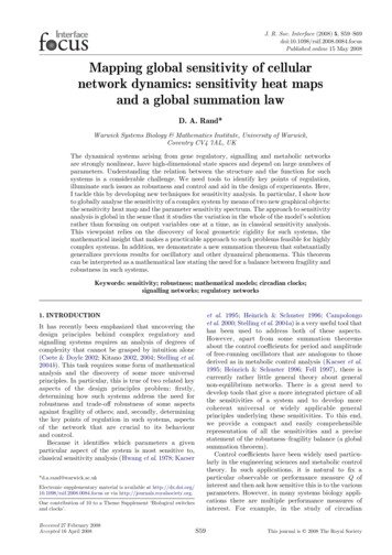
S60Mapping global sensitivityD. A. RandTable 1. A list of some models analysed together with the number of state variables n, the number of parameters s and the rate ofdecay a of the singular values si (i.e. log10 si wKai). (The superscripts ‘u’ and ‘f’ for the circadian oscillators indicate,respectively, the values for the cases where the oscillator is unforced and forced by light.)modelnsaNeurospora clock; Leloup et al. (1999)Drosophila clock; Leloup et al. (1999)Drosophila clock; Ueda et al. (2001)Drosophila clock; Tyson et al. (1999)mammalian clock; Leloup & Goldbeter (2003)mammalian clock; Forger & Peskin (2003)yeast cell cycle; Tyson et al. (2002)full NF-kB model; Hoffmann et al. (2002) and Nelson (2004)glycolytic oscillations; Ruoff et al. .44— the sensitivity heat map (SHM ) from which one is ableto effectively identify those observables Q that aresensitive to some parameter, and— the parameter sensitivity spectrum (PSS ) that characterizes the sensitivity of these observables and thesystem as a whole with respect to each parameter.The crucial observation that makes the theoryapplicable in practice by ensuring that for a giventolerance the above objects are compact and manageable is that such network systems are rigid in thefollowing sense. The map from parameters to thecorresponding solutions of interest (a map from ahigh-dimensional space Rs to an infinite-dimensionalsolution space) locally maps round balls to ellipsoidswith axes lengths s1 R s2 R s3 /Rss where the lengthssi decrease very rapidly. This is rigidity becauserandom jiggling of the parameter vector in the highdimensional parameter space results in the variation ofthe solution of interest that effectively occupies a spaceof much lower dimension.J. R. Soc. Interface (2008)0–1–2log10oscillators one is interested in many aspects such as thefree-running period, the strength of entrainment andthe consequent phases of the various molecularproducts, the phase response curves, period and phaseas a function of temperature and the response todifferent day lengths. For signalling systems such asthat of the NF-kB system, one is interested in multipleaspects of the response to a signal related to itsstrength, timing, persistence, decay and transient,equilibrium or oscillatory structure. Moreover, in thesearch for key points of regulation there may be aspects,where the system is particularly sensitive, that do notcorrespond to obvious performance measures. Therefore, it would be extremely useful to have an effectiveapproach that will find the sensitivity of all theperformance measures and operating aspects of agiven model.The approach to sensitivity analysis developed here isa global one that studies the variation of the wholesolution rather than focusing on just one output variable.In addition, this more global approach allows us toaddress which observable variables Q (henceforth calledobservables) are affected by which parameters k j withouthaving to choose the variable or parameter in advance.The results of this analysis can be summarized in–3–4–52468index101214Figure 1. The plot shows log10 si for the largest singular valuesof the models in table 1. The case shown is for relative changesin both parameters and the solution (as explained in §2.4). Wesee that, for all these examples, the si decay exponentially likeexpðKaiÞ and that the rate of decay aO0 varies significantlyfrom model to model. The models are listed in the same orderas in table 1, which are as follows: open circle, Neurospora;open square, Drosophila 1; open diamond, Drosophila 2;open down triangle, Drosophila 3; open up triangle, mammalian 1; filled circle, mammalian 2; filled square, cell cycle;filled diamond, full NF-kB; filled down triangle, glycolyticoscillations.The sensitivity principal components (PCs) Ui(t)that we present in §2 are key components of our theory.These are multidimensional time series from which allsystem derivatives can be calculated and whose importance rapidly decreases as i increases. We show that,when the parameters being varied are a full set of linearparameters, the sensitivity PCs satisfy a global summation theorem which says that a certain linearcombination of them sums to a function that is simplyrelated to the original differential equation. This globalsummation theorem contains within it the other knownsimple summation theorems for dynamic systems suchas those for the period and amplitude of an oscillatorysolution of an unforced oscillator. However, it is asubstantial generalization because it relates a set offunctions rather than a set of numbers and thus iseffectively an infinite number of simple summationconditions. Moreover, unlike the classical summation
Mapping global sensitivity(a)ratio max1.00 5.171.00 0.860.98 0.700.93 0.680.51 –0.130.31 0.070.25 0.430.13 6.100.12 6.180.12 3.600.09 1.470.06 0.050.04 –0.010.01 0.04 0.01 0.00 0.01 0.01CRYcyto PER : CRYnuc PER : CRYPer mRNAPERBmal1 mRNAnuc BMAL1cyto BMAL1P: C :C:BCry mRNACRY-pnuc PER : CRY-pPER-pnuc BMAL1-pcyto BMAL1-pcyto PER : CRY-p051015time/phase (h)20051020D. A. 8(b)420–215time (h)Figure 2. C1(t)Zs1U1(t) for the model of the mammalian circadian clock due to Leloup & Goldbeter (2003) with no forcing bylight (i.e. in DD). Each of the 16 components C1,mZs1U1,m is represented by a coloured strip that shows the value of C1,m(t) atthe corresponding time 0%t%T, where T is the period of the oscillation. In order to highlight their structure the C1,m are scaledby a factor 1/am so that the values taken by C1,m(t ) fill a maximal range of the interval from minm 0 ,tC1,m 0 (t) to maxm 0 ,tC1,m 0 (t).They are shown in order of decreasing am and the values of am are shown in the column headed ratio. Thus one sees that theamplitude am of C1,m for CRY protein is more than 100 times that of phosphorylated cytoplasmic PER CRY complexes orphosphorylated cytoplasmic BMAL1 protein. A glance shows that CRY is the most sensitive in that am is largest, followed bycytoplasmic PER CRY complexes (cyto PER:CRY), nuclear PER CRY complexes (nuc PER:CRY), Per mRNA and PERprotein in that order. We can also quickly see at what times or phases these variables are fragile or robust. Thus we see that CRYis most fragile at times close to tZ14.5 hours and relatively fragile over a broad band of phases centred on this time, while thevariable for nuclear PER CRY complexes is most fragile close to tZ18 hours, but even there, much less so than CRY. Onthe other hand since their amplitude is so small, the last six variables are relatively insensitive at all phases. In calculating thesesensitivity PCs no scaling of the dynamical variables is carried out but the scaled parameters hjZlog kj have been used. In caseswhere these variables have significantly different scales, it is usually preferable to scale the variables to concentrate on relativechanges rather than absolute ones. As is explained in §3, this scaled approach is very easy to implement. In (b), the curves are asfollows: dark blue, CRY; green, cyto PER:CRY; red, nuc PER:CRY; light blue, Per mRNA; purple, PER.theorems, it applies to non-autonomous systems suchas forced oscillators as well as to autonomous systems.I have applied the theory to a broad range of examples(table 1), but for the purposes of discussion andillustration in this paper we will mainly consider tworepresentative examples: a model of the mammaliancircadian oscillator (Leloup & Goldbeter 2003) and aversion of the Hoffmann model for the NF-kB signallingsystem (Hoffmann et al. 2002). The former is a reasonablyrepresentative example of a periodically oscillatingsystem and for the latter the solution of interest is atransient solution produced by an incoming signal.2. RESULTSSuppose we are considering a regulatory or signallingsystem modelled by the differential equationdxZ f ðt; x; kÞ;ð2:1Þx ZdtJ. R. Soc. Interface (2008)where t is time; x Z ðx 1 ; .; xn Þ are the state variables ofthe system; and k Z ðk 1 ; .; ks Þ is a vector of parameters.The vector k may contain all the parameters but we willalso consider the case where it only contains some andwhere the other parameters are held fixed and onlyk 1 ; .; ks are varied. For example, k may consist of justthose parameters that the system is particularlysensitive to or may consist of just the linear parametersas defined in §2.5.In general, there will be a solution x Z gðt; kÞ or a classof solutions defined for a specific time range 0% t% Tthat are of particular interest. For example, for circadianoscillations the primary object of interest is an attractingperiodic orbit of equation (2.1) and T will be the periodof this orbit. On the other hand, for models of signallingsystems, one is often interested in a solution that is notperiodic but is defined by a given initial condition x 0.Such a signalling system is usually also subject to a givenperturbation caused by an incoming signal and this
S62Mapping global sensitivityD. A. Randwill typically be modelled by a sudden change in asystem parameter or by the time dependence of the r.h.s.f ðt; x; kÞ of equation (2.1).In regulatory and signalling systems, the values of twoparameters may differ by an order of magnitude or more.Therefore, it is usually not appropriate to consider theabsolute changes in the parameters k j, but instead toconsider the relative changes. A good way to do this is tointroduce new parameters hj Z log kj because absolutechanges in hj correspond to relative changes in k j. Then,for small changes dk to the parameters, dhj Z dkj kj , sothe changes dhj are scaled and non-dimensional.2.1. Fundamental observationThere are two aspects to the fundamental observationbehind the tools and analysis presented here. The first isthat for such regulatory and signalling systems there arethe following easily computable objects:(i) a set of n-dimensional time series Ui ðtÞ Z ðUi;1 ðtÞ;.; Ui;n ðtÞÞ, i Z 1; .; s defined for 0% t% T,which are of unit length and orthogonal to eachother in the sense of equation (2.3),(ii) a decreasing sequence of s positive numberss1 R/R ss called sensitivity singular values, and(iii) a special set of new parameters lZ ðl1 ; .; ls Þthat are related to the original (scaled) parametervariations dh by anPorthogonal linear transformation W (i.e. li Z j Wij dhj ),with the following key property that connects them: ifdh is any change in the (scaled) parameter vector thenthe change dg in the solution g of interest is given byXli si Ui ðtÞ C Oðkdhk2 Þ:ð2:2ÞdgðtÞ ZiThe second aspect is that for a broad range ofnetworks such as those in table 1, the amplitudess1 R/R ss R 0 actually decrease very rapidly, usuallyexponentially in the sense that log si decreases linearlywith i, i.e. si wexpðKiaÞ, aO0.The Ui are of unit length and orthogonal to each otherin the following sensen ðTXUi;m ðtÞUj;m ðtÞdt Z dij ;ð2:3ÞmZ1 0where dij Z 0 if isj and equals 1 if iZj. These are calledsensitivity PCs.We stress two points here: (i) that the given systemand solution of interest determine the Ui , the si , W andthe li and (ii) that the change dg is described by (2.2) interms of these for any parameter perturbations dh.It can easily be shown (see the electronic supplementary material) that the derivatives vg vhj of thesolution g with respect to the parameters hj are given bysXvgZSij Ui ;vhji Z1ð2:4Þwhere Sij Z si Wij .One can regard equation (2.3) as saying that Ui andUj (isj ) are uncorrelated as functions of time t. TheJ. R. Soc. Interface (2008)derivatives vg vhi and vg vhj will in general becorrelated with each other and writing them as inequation (2.4) is a decomposition of them into uncorrelated time series. Since the si decay rapidly from asignificant value we see that, in fact, the derivatives arehighly correlated and their correlation is concentrated ina few components Ui with low values of i.The usefulness of the Ui , the si and the Sij arises froma combination of the following facts:(i) they are straightforward to compute (see §3),even for very complex models,(ii) classical sensitivity coefficients can be expressedin terms of them,(iii) when represented in a heat map (see below), onecan rapidly map out all the sensitivities of acomplex model, and(iv) since the amplitudes si get small very quickly, fora broad class of network models it is usuallynecessary to consider only a small number of thedominant Ui.Let us illustrate the fundamental observation byconsidering the two models mentioned above. For themodified Hoffmann model (Hoffmann et al. 2002), thereare nZ10 state variables x 1 ; .; x10 corresponding to theconcentrations of nuclear and cytoplasmic NF-kB andIkBa and their complexes plus IKK, and sZ42parameters kj most of which are rate constants. This isa simplified version of the model in Hoffmann et al.(2002) in which, of the IkB’s, only IkBa is includedand not IkBb and IkB3. The solution g(t) consideredis the transient orbit produced when an incomingsignal at tZ0 increases the level of IKK above theequilibrium level. The IKK is washed out at tZ600 min.The mammalian clock model (Leloup & Goldbeter 2003)has nZ16 state variables and sZ53 parameters. Bothhave rapidly decreasing sensitivity spectra as is shownin figure 1. The s1-scaled sensitivity PC C1 ðtÞZ s1 U1 ðtÞfor the above model of the mammalian oscillator isshown in figure 2 as a heat map. Although these twomodels have a large number of state variables andparameters, to study all their sensitivities that are nosmaller than 5% of the biggest it is enough to consideronly the first five Ui.The results behind this observation about the rapiddecay of the si were first developed independently inBrown & Sethna (2003), Brown et al. (2004) and Randet al. (2004, 2006). In the former work, the si appeared asthe square roots of the eigenvalues of the Hessian ofthe function that has to be minimized when doingleast-squares fitting of parameters to data for suchmodels. In the latter reference they arose as part of anargument about the complex structure of circadianclocks being a result of the inflexibility of such systemsdespite the large number of parameters. The linkbetween these two approaches is provided by the matrixS Z ðSij Þ defined above (see equation (2.4)) bySij Z si Wij . The square S t S is an example of a Fisherinformation matrix and its eigenvalues are the s2i . It canbe shown that under certain conditions it is the meanvalue of the abovementioned Hessians (see electronicsupplementary material). In Waterfall et al. (2006), it is
Mapping global sensitivityargued that such systems form a universality class and itwill be important to determine whether this is true orwhether there is a more mundane reason for this decay.More evidence for the seemingly universal ubiquity ofthe rapid decay of the si in tightly coupled systemsbiology models and the consequences for parameterestimation are discussed in Gutenkunst et al. (2007).2.2. Classical sensitivity coefficients from the UiTypical classical sensitivity coefficients can be written interms of the Ui and Sij. As explained in the electronicsupplementary material many can be written either asa sumCQjv log Q1 vQ1 XZZZa D ðt Þv log kjQ vhjQ [ [ j;m [ð2:5Þfor some finite set of times t[ or as an integral over ainterval of times t1 % t[ % t 2ð1 t2CQZaðt[ ÞDj;m ðt[ Þdt[ ;jQ t1where Dj;m ðt[ Þ is eitherXSij Ui;m ðt[ Þ oriXSij U i;m ðt[ Þ;ð2:6Þiand U i;m is the derivative of Ui,m with respect to time t.Examples involving a sum include the control coefficients of phase and amplitude for forced oscillators andthe time for signals to peak in signalling systems.Examples involving an integral include the Fouriertransforms of the components of the solution (reflectingchanges in the shapes of the time series). Thus, weconclude that the control coefficients of interest are alllinear sums or integrals over t[ of terms that are of theform given in (2.6). This fact is key to understanding theuse of the SHMs.In the electronic supplementary material the readerwill find a table listing some key observables foroscillators and signalling systems and giving theexpressions for their control coefficients in terms of theUi,m using formula (2.5).2.3. SHM and parameters sensitivitiesgraphically summarize all the system’ssensitivitiesWe now discuss how to analyse the sensitivity of such acomplex dynamical system globally using the SHM andthe PSS (figures 3 and 6). They allow us to graphicallyanalyse what observables are significantly changed bywhat parameters. We do not have to fix the observableor parameter in advance but let the model decide whatthe most salient observables are. The SHM and PSS areintrinsic to the system and characterize its sensitivity ina global fashion.The strategy is to(i) use the SHM to identify all those times t[ andindices i and m that correspond to the terms,which are significantly large, of the form given inJ. R. Soc. Interface (2008)D. A. RandS63equation (2.6) and thus to effectively determinewhich observables Q have C Qj significantly largefor some parameters k j, and then to(ii) use the PSS to identify, for those Q from (i), whichof the parameter indices j have C Qj significantlylarge.2.3.1. Sensitivity heat map. Suppose jWij j jU ðtÞjfi;m ðtÞ Z si maxi;mjand ðd ÞjWij j jU ðtÞj:fi;m ðtÞ Z si maxi;mjð2:7Þð2:8Þðd Þfi;m ðtÞZ j f i;m ðtÞj,si are decreasing(Note thatmaxj jWij j% 1, jUi;m ðtÞjrapidly for the systems%1 and theof interest.)PPPThen j i Sij Ui;m ðtÞj% i fi;m ðtÞ and j i Sij U i;m ðtÞjP ðd Þ% i fi;m ðtÞ. Thus, if C Qj is a linear combination of termsas in equation (2.6) using a given m and a given set ofðdÞtimes t[, the following is true: if fi;m ðt[ Þ and fi;m ðt[ Þ areQsmall for all those values of t[, then jC j j must be small.Therefore to determine which observables can have asignificant control coefficient C Qj we need to determineðdÞall i, m and t[ such that either fi;m ðt[ Þ or f i;m ðt[ Þ havesignificant values. To do this we fix a small threshold t(e.g. 1% of the maximum value achieved by all the fi,mðdÞand fi;m ) and identify all pairs (i,m) such that eitherðdÞmaxt f i;m ðt[ Þ or maxt f i;m ðt[ Þ is greater than t. Luckily,since these sizes are comparable to si , there areðdÞrelatively few pairs (i,m) for which fi,m or fi;m have tobe plotted: in the examples studied so far about twice thenumber of state variables.ðdÞThese fi,m and fi;m are then plotted in the SHM. SinceðdÞrelatively few fi,m or fi;m have to be plotted, the heat mapis compact and therefore convenient. For each such pair(i,m) we inspect the fi,m plotted in the SHM to determineðdÞthe set Ti,m of times such that fi,m(t) or fi;m issignificantly large. This achieves step (i) above.SHMs for the mammalian clock model and the NF-kBsignalling systems are shown in figures 3 and 6.2.3.2. Parameter sensitivity spectrum. The matrixSij Z si Wij characterizes the sensitivity of the systemwith respect to each parameter. Recall that, up tosecond-order terms that are Oðjjdhjj2 Þ, the variation dgproduced by a parameter variation dhZ ðdh1 ; .; dhs Þ isXXdgðtÞ Zvg vhj ðtÞdhj ZSij Ui ðtÞ dhj ;ji;jPsince vg vhj ðtÞZ i Sij Ui ðtÞ. We see that Sij completelydetermines the effect of small changes dhj in the jthparameter hj. Moreover, since the Ui(t) are orthogonal intime-series space, the Sij act in independent directionsand efficiently parametrize the derivatives vg vhj . Infact, the Sij give a representation of the derivatives thatis optimal in that it maximizes the effect of terms withlow i (for a precise statement see the electronicsupplementary material).
S64Mapping global sensitivityD. A. Rand(a) 0.080.050.06CRYcyto PER : CRYnuc PER : CRYPer mRNAPERCry mRNABmal1 mRNACRY-pnuc BMAL1-pnuc PER : CRYBmal1 mRNAcyto PER : CRYPer mRNACRYP:C:C:Bcyto BMAL1nuc BMAL1PERCry mRNAnuc PER : CRYCRYcyto PER : CRYPer mRNACry .360.330.270.200.140.160.210.130.08Per mRNAcyto PER : CRYnuc PER : CRYCRYCry mRNAPERnuc BMAL1Bmal1 mRNACRY-pP:C:C:Bnuc PER : CRY-pPer mRNACRYnuc PER : CRYcyto PER : CRYnuc BMAL1P:C:C:BCry mRNABmal1 mRNAPer mRNACRYCry mRNAcyto PER : CRYnuc PER : CRYPer mRNACRYPer mRNACry .210.140.07200– dÞFigure 3. (a) The SHMs for the model of the mammalian circadian clock discussed in figure 2: (i) fi,m and (ii) fi;m . TheðdÞthreshold for the fi,m is set to be 5% of the global maximum of the fi,m(t). For the fi;m (t) heat map, the correspondingthreshold is 7.5%. These were chosen to keep the figure size small and smaller thresholds can be used. The only values of iðdÞ(the sensitivity PC index) and m (the variable index) for which maxt fi,m(t) or fi;m (t) is greater than this threshold have iZ1,2, 3, 4 or 5. Each block of variables corresponds to one value of i. Thus, in (i), the first block of nine variables corresponds toiZ1. The plotted fi,m are coloured on the scale shown after scaling each of them by a factor 1/ai,m to make all theiramplitudes the same as that with maximum amplitude. These factors ai,m are in the column marked ratio. (b) The PSS whereeach group of bars corresponds to the value of log10 jSijj for a particular parameter k j. These are only plotted for those i forwhich jSij j is significant (in this case iZ1–4). They are coloured as follows: red (pc 1), iZ1; blue (pc 2), iZ2; green (pc 3),iZ3; light blue (pc 4), iZ4. The parameters k j are ordered by maxiZ1–4jSijj and only the 25 most sensitive are plotted. Todemonstrate how the heat maps can be used, we consider the sensitivity of the 32 phases of the maxima and minima of thevarious products. We see from table 1 of the electronic supplementary material that the control coefficient of such a phase forxm(t) is proportional to a linear sum of the Wij C i;m Z Sij U i;m , and we therefore need to check whether the phases of theðdÞðdÞmaxima or minima are hot times for the fi;m . We have therefore plotted the maxima and minima on the fi;m heat map (black,minima; white, maxima). We immediately see that some of the maxima are sensitive, notably Per mRNA and cytoplasmicPER–CRY complexes that are the most sensitive. Following these, approximately one-third as sensitive are nuclear PER–CRY complexes, Cry mRNA and CRY protein. Of the minima, only those of cytoplasmic PER–CRY complexes and CRYprotein appear to be significantly sensitive. Using the software described in the electronic supplementary material, one canðdÞquickly turn this into quantitative information. For the most sensitive phases f, the high values of fi;m ðfÞ occur when iZ1.Therefore, to see what parameters these most sensitive phases are sensitive to, we check the red bars in the PSS in the secondrow of the figure, since these are the values of log10 jS1j j. We quickly see that four parameters dominate (vsp, vsc, vmp andkib) and three others have a sensitivity a little above 10% of the maximum. Only 12 out of the 56 parameters have more than1% of the maximum sensitivity for these phases.In figure 4 we see that, for the model of themammalian circadian clock, the magnitude of the Sijdecreases rapidly with i and relatively few of them havelog10 jSij jO 10K3 . In figures 3 and 6, the log10 jSij j areplotted as a grouped bar chart with the parameterskj reordered according to the size of their sensitivity.Using this for a given value of i we can immediatelyidentify the strength of each parameter in movingthe solution g in the direction of Ui. Although notmonotonically decreasing in i, the Sij neverthelessrapidly get small as i increases. This can be seen infigure 4 where we plot log10 jSij j and see that very few ofJ. R. Soc. Interface (2008)the Sij have a magnitude greater than one per cent ofmaxij jSij j. Therefore, we only have to consider the Sij fora few values of i and the grouped bar chart can berestricted to these.Thus, if we (i) use the SHM to determine the set Ti,mðdÞof times t such that either fi,m(t) or fi;m ðtÞ is significantlylarge, and (ii) use the PSS to identify those parameters hjsuch that jSijj is significantly large we obtain a set oftriples (i,m,j ) that give the significant terms of the formin equation (2.6). These are called hot. We can thenconclude that the control coefficients C Qj that aresignificant are those which involve terms of the form
Mapping global ��3D. A. RandS65For the purposes of illustration let us suppose that weare interested in the first two oscillations (i.e. untiltZ200) and in the full trajectory (i.e. until tZ1000).We see from figure 5 that the different componentsgi(t) of the solution gðtÞZ ðg1 ðtÞ; .; gn ðtÞÞ have verydifferent amplitudes. This raises the problem thatparameter changes will tend to produce larger absolutechanges to those variables with larger magnitudes.Therefore, it will usually be the case that, in situationslike this, relative changes in the gi are more appropriatethan absolute ones. One way to allow for this is to uselog gi ðtÞ instead of gi ðtÞ. However, this is not sensible inthis case as for some times t, gi(t) is very c
and a global summation law D. A. Rand* Warwick Systems Biology & Mathematics Institute, University of Warwick, Coventry CV4 7AL, UK The dynamical systems arising from gene regulatory, signalling and metabolic networks are strongly nonlinear, have high-dimensional state spaces and depend on large numbers of parameters.