WIXLIB

This leads to a stylised representation of the balance sheet, shown in Table 1.The difference between total assets and total liabilities is represented by the firm’sequity E.We further discuss in Section 3 the mapping of balance sheet data and regulatory data to the format presented in Table 1.AssetsIlliquid assets:(i) Subject to margin requirements, I(ii) Not subject to margin requirements, JMarketable assets:(i) Subject to margin requirements, M(ii) Not subject to margin requirements, NLiquid assets, CLiabilities and equityCurrent liabilities, SLong-term liabilities, LCapital (equity), ETable 1: Stylised balance sheet of a financial institution.2.2Dynamics of balance sheet components under stressWe now describe the dynamics of balance sheet components in a stress scenario. Itis helpful to represent the sequence of transformations of balance sheet componentsas a two-period model, as in Figure 2.t 0Shock to assets: I, J, M, N- Initial balance sheett 1 Effect on liquidity: t 2 C, S- Expected cash flows- Margin calls- Credit gradeLiquidity management:- Short-term borrowing- Asset salesFigure 2: Evolution of balance sheet components.Consider a leveraged financial institution with a balance sheet as in Table 1.We denote by I0 , J0 , M0 , and N0 the initial value of balance sheet components,the subscript 0 indicating their initial value at t 0. The initial value of currentliabilities S0 represents the amount of liabilities maturing at t 2, while L07

represents the amount of liabilities maturing after t 2. C0 denotes the currentlevel of cash reserves and balances with central banks.We now consider the impact of an adverse market scenario on this balancesheet.Stress scenarios are typically defined in terms of shifts to risk factors suchas real GDP, interest rates, credit spreads, equity prices, exchange rates, andother economic variables to which portfolio components are sensitive. Denotingby X (X1 , ., Xd ) these risk factors, each stress scenario may be described interms of shocks X ( X1 , ., Xd ) to risk factors.Direct impact on solvency The reaction of portfolio components to such astress scenario is evaluated using models calibrated to the risk structure of theportfolio. The models used to derive stress impacts differ across default shocksand market shocks. While the effect of default shocks on credit exposures maytake time to materialize, market shocks immediately affect the fair valuation ofmarket exposures. To produce an integrated risk modelling framework, we assumethat firms assess the impact of default shocks on equity using a forward-lookingapproach (rather than an incurred loss method), and thus the horizon over whichshocks hit P&L is the same across risk types. This view is consistent with BaselIII regulatory framework for internal-ratings based models, and the newly implemented accounting IFRS 9 provisions2 .For credit shocks, defaults are considered in lending positions (in general valued according to accrual accounting), traded credit positions (“issuer default”,positions measured at fair values) and counterparty exposures like OTC derivatives and Securities Financing Transactions. Impairment losses reduce the carryingamount of credit risk positions affecting the value of equity. Impairment chargescan be computed as the impact of stressed credit risk parameters i.e. probabilityof default (PD), loss given default (LGD), and exposure at default (EaD), on theinitial value of the position. Shifts to PDs, LGDs, and EaDs can be expressed interms of sensitivities to underlying risk factors.For market risk shocks, the impact of the shocks on the fair values of theunderlying positions can be measured either by revaluation of the positions in theportfolio under the stress scenario (full valuation method) or, as done frequentlyin regulatory stress tests, by using a linear approximation of the dependence ofportfolio components with respect to risk factors, in terms of sensitivities to risk2To compute regulatory capital, banks using internal-ratings based models for credit risk takea forward-looking approach to determine capital ratios. From an accounting perspective, IFRS9 requires loan allowances based on 12 month expected losses if the credit risk has not increasedsignificantly, and expected lifetime losses for exposures that have deteriorated significantly.8

factors.The impact of market risk on bank portfolios at partial or full fair value measurement is typically assessed via a full revaluation after applying a common setof stressed market risk factor shocks in firm internal stress tests and regulatorybottom-up stress tests or, in a regulatory top-down approach, using a linear approximation based on sensitivities to risk factors. Denoting k A the sensitivityof balance sheet component A to risk factor Xk , the change in the value of thisbalance sheet component in the risk scenario is then given by A d k A. Xk A. X,(1)k 1where M denotes the vector of sensitives of balance sheet component M . Similarly we may compute the changes in balance sheet items I, J, N as I I. X, J J. X, M M. X, N N. X. (2)These sensitivities may be computed using satellite models linking scenario shocksto credit risk parameters (default shocks), or calculating the impact of risk factorson fair-valued positions using the delta method (market shocks).3Impact on liquidity Liquidity risk arises from the uncertainty to meet paymentobligations in a full and timely manner in a stressed environment. In the model,obligations coming due at t 2 include four components.1. Unconditional liabilities: these are liabilities maturing at t 2. Their sizecorresponds to current liabilities and hence is denoted by S0 .2. Expected cash-outflows: these include contractual cash-flow obligations (e.g.interest payments on interest-bearing liabilities, coupons, operating costs),projected outflows from non-maturing liabilities (e.g. sight, operational deposits) and estimated drawdowns from undrawn credit and liquidity lines.Denoting these outflows by ECO, the stable component of short-term liabilities payable at t 2 can then be expressed asS1 S0 ECO.(3)3. Contingent liquidity risks: firms post and receive collateral to support orreduce the counterparty credit risk (CCR) relative to derivative transactionsor to securities financing transactions, including transactions cleared through3See Section 3 for more details.9

a central counterparty (CCP). Here we focus on liquidity needs from changesin the value of collateral posted by the bank (e.g. in repo transactions) ratherthan on collateral received (e.g. in reverse repos) to allow an integratedassessment of the solvency and liquidity risk of the firm from valuation shocksto the bank assets. For assets subject to variation margin, negative changesin asset values lead to margin calls that add to current liabilities, which wedenote by S ( I) ( M ) ,(4)whereas positive changes generates margin calls to the counterparty, whichlead to cash inflows expected at t 2, and which we denote by C ( I) ( M ) .(5)The interaction between solvency and liquidity risk through margin requirements and creditor runs may lead to a severe amplification of losses in astressed environment. In a derivative transaction or securities financingtransaction with no margin payments, although both sides may mark-tomarket their position daily, there is no exchange of cash flows: any lossesor gains purely affect the solvency of the institution. In this case, capitalbuffers are an adequate tool to address any risk externalities. On the otherhand, if an asset is subject to margin requirements, this creates a liquidityoutflow in the form of a variation margin payment. As a result, such shocknot only affects the solvency of the institution but also its liquidity by drawing on the held cash reserves with an immediate effect (typically within fewdays), since all payments are done in cash or liquid assets.4. Credit downgrades and credit-sensitive funding: The direct impact of theshocks described above on the firm’s equity is given byE1 E0 I J M N C1 S1 L0 .(6)If due to these losses the firm’s equity falls below a threshold, then the firmmay be subject to a credit downgrade. We assume such a downgrade occursif the leverage ratio exceeds a level δ i.e.I1 J1 M1 N1 C1 δ.E1(7)Such a downgrade may trigger a contingent cash outflow SD through the lossof credit sensitive funding, depositor runoffs, failure to roll over short termdebt or margin calls associated with a credit downgrade. We denote by SDthe increase in current liabilities resulting from a downgrade.10

As a result, conditional on the stress scenario, current liabilities due at t 2increase toS2 S1 S SD 1downgrade .(8).On the other hand, the reserve of liquid assets is increased by the expectedcash-inflows from contractual claims (e.g. interest payments) and maturing assetswhich are not reinvested (e.g. inflows from performing exposures and securedlending). Denoting this amount by ECI we have thatC1 C0 ECI(9)Mitigating actions At t 1, if liquid assets are not enough to cover conditionalcash outflows (expected and unexpected), the bank can undertake mitigating actions (from its contingency funding plan and recovery plan) to cover the liquidityshortfall λ which we define formally asλ (S2 {C1 C}) .(10)In the short term, a financial institution has access to three sources of funding,stated in a usual order of preference:1. Unsecuritized borrowing: we assume the financial institution to have accessto short-term unsecuritised loans given at an exogenous market interest raterU . This access depends on the firm’s creditworthiness: we assume that thefirm’s access to such funding ceases once it has been downgraded. Furthermore, the distance to downgrade leads to an upper bound on the volume ofunsecuritised lending available to the firm:vU (E1 δ {I1 J1 M1 N1 C1 }) .(11)In other words, we assume that the highly leveraged institutions are considered more risky on the market, and hence can access a smaller pool ofliquidity than lesser leveraged firms. Subject to this constraint, the amountof money a financial institution will borrow through this channel can beexpressed asBU min{λ, vU }.(12)2. Repurchase agreements (repo): in contrast to unsecuritised borrowing, therepo market requires the provision of liquid marketable (unencumbered) collateral as a form of security. The amount vR of funding which may be raised11

through this channel available is limited by the firm’s pool of unencumbered marketable assets, discounted by the corresponding haircut parameterh [0, 1), that isvR (1 h)(M1 N1 ).(13)Consequently, the amount of cash that a financial institution will raisethrough repo market is then given byBR min{λ BU , vR },with an associated borrowing cost given by the (exogenous) repo rate rR .3. Liquidation of assets (fire sales): we assume that in the short-term a liquiditystressed financial institution can only sell a fraction θ [0, 1] of its illiquidassets in a fire sale for an associate price discount ψ [0, 1). Note that onlyunencumbered illiquid assets (not subject to margin requirements) can bemonetized in a fire sale. In other words, the maximum amount of liquiditythat can be raised in a short-term can be expressed asvF ψθJ1 .(14)The fraction θ depends for example on the available market liquidity andthe length of sales horizon. Consequently, we expect θ to be small in a stresstest scenario. Similarly, we usually think of the associated fire sale discountto be large (in excess of 50%).These mitigating actions increase the liquidity buffer of the bank at t 2 toC2 C1 C BU BR ωvF ,(15)where BU represents the amount of new unsecuritised borrowing, similarly BR isthe amount borrowed on the repo market, and ω [0, 1] is an endogenous fractionof liquidated assets in a fire-sale for a price discount of ψ [0, 1) such that{}(S2 (C1 C BU BR )) ω min,1 .ψθJ1The amount of long-term liabilities rises by the amount of new liabilities fromunsecured and secured funding, and declines by the cash-flow amount due to creditrisk sensitive funding, that isL2 L0 (1 rU )BU (1 rR )BR SD 1downgrade .(16)As a consequence of these mitigating actions, the value of equity falls toE2 E1 rU BU rR BR ω(1 ψ)θJ1 .12(17)

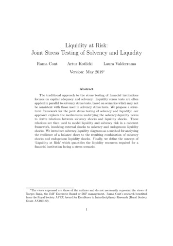
Insolvency and illiquidity A financial institution is deemed insolvent whenthe equity falls below a certain threshold, here taken without loss of generality tobe zero. That is, a firm fails due to insolvency when E2 0. It is said to be illiquidwhen current liabilities exceed the firm’s capacity to raise liquidity i.e. C2 S2 ,where C2 is the available liquidity, given by (15) and S2 are the current liabilitiesdue at t 2, given by (8). It is possible for a firm to be illiquid without beinginsolvent, as it is possible to be insolvent without being illiquid.The summary of dynamics of balance sheet components in our model is givenby Figure 3.Figure 3: Joint stress test of solvency and liquidity.2.3Solvency-liquidity diagramsThe sequential dynamics of the balance sheet in a stress scenario may be visualizedin the form of a solvency-liquidity diagram in which the financial institution’s equityis represented on the horizontal axis and its liquidity resources on the vertical axis(see Figure 4).A solvent and liquid institution corresponds to a point in the upper rightquadrant (first quadrant). The vertical coordinate corresponds to its liquiditybuffer while the horizontal coordinate correspond to the firm’s equity.13

Figure 4: Solvency-liquidity diagram describing the behaviour of a balance sheetin a stress scenario.A loss in asset values in a stress scenario moves this point to the left. Depending on the cash flows arising in the stress scenario, we will also have a verticaldisplacement upwards (if there is net incoming cash, for example due to variationmargin and interest received) or downwards (if there are net outflows, for examplefrom margin and interest payments).Failure occurs when the institution exits this first quadrant. If it crosses thehorizontal axis (see Figure 5a), this corresponds to an illiquidity induced default,while if it crosses the vertical axis (see Figure 5b) this corresponds to failure dueto insolvency. The distance to the axes represents the capital and liquidity buffers(see Figure 4).An adverse stress scenario leads in a ’south-west’ shift on the diagram: theprecise direction of the shift depends on balance sheet sensitivities, while the sizeof the shift corresponds to the severity of the shock. A pure solvency shock drawson the capital buffer without affecting the firm’s liquidity reserves, and hencecorresponds to a horizontal shift on the solvency-liquidity diagram. On the otherhand, a pure liquidity shock caused by a run of creditors or a failure to rollovershort-term debt due to downgrade corresponds to a vertical shift on the diagram.For a fixed adverse market scenario, the loss in equity due to the shock is independent of the balance sheet composition in terms margin requirements. However,14

as the proportion of assets subject to variation margin increases, the reduction inliquidity position of a financial institution also increases. In that case, it becomesmore likely that the firm becomes illiquid while still solvent as the shock severityincreases.15

(a) Illiquidity induced default.(b) Insolvency induced default.Figure 5: Examples of scenario analysis using solvency - liquidity diagrams. (a)Stress scenario leading to illiquidity. (b) Stress scenario leading to insolvency.16

3Mapping of balance sheet variables and liquidity templatesThe purpose of this section is to show how balance sheet information –especiallyin the format of templates available to regulators– may be mapped to the formatshown in Table 1 used as an input for our stress testing approach. In this sectionwe describe how to use various data sources to generate the inputs required in ourframework. We then provide a numerical illustration using publicly available datafor a global systemically important bank (G-SIB).3.1Data requirementsOur stress testing approach requires two types of inputs: Balance sheet data, with sufficient granularity in order to extract the categories displayed in Table 1. Market data and risk parameters to be used for estimating the profit andloss (P&L) of various portfolio components in the stress scenario.These requirements are not very different from the inputs of current solvency stresstests but require the data to be formatted in a slightly different way, as discussed inSection 2. Central banks and regulators typically have access to data on portfoliopositions, risk parameters, pricing models and methodologies to assess sensitivitiesto stress. For instance, in the European reporting framework, financial data iscollected in FINREP templates while risk data is submitted in COREP templates.The reporting requirements, defined by the European Banking Authority (EBA)via the implementation of technical standards or guidelines, are complementedwith short-term exercise ad-hoc data requests which collect additional granulardata on complex portfolios including sensitivities to moves in market risk factors.Our stress testing framework requires this data to be available at a sufficientlygranular level to derive the above information for each component of the balancesheet.Table 2 summarises the mapping of asset categories observed in regulatory andaccounting templates to balance sheet components required in the model. Assetsare classified as ’marketable’ or ’illiquid’. Marketable refers to the availability ofthe assets for raising short-term funding in a stress scenario, either through arepurchase agreement or sale. Such assets therefore need to be unencumbered byother repurchase agreements. Since we are interested in behaviour of the balancesheet under stress, we restrict marketable assets to those which can be used forGeneral Collateral (GC) financing. Loans, non-GC assets, physical assets andheld-to-maturity assets are typically classified as illiquid in our setting.17

IlliquidassetsMarketableassetsLiquidassetsNot subject to variation marginLoansHeld to Maturity and non-GC AssetsPhysical assetsUnencumbered assets (General collateral):(i) Held for trading(ii) Financial investmentsEquityCash unencumberedReverse reposSubject to variation marginNon-standard OTC derivativesEncumbered assetsExchange-traded derivativesStandardized OTC derivativesTable 2: Mapping of common asset classes to the model input format.Once the balance sheet data has been mapped to the format shown in Table 2, the stress test requires to estimate the variations in each compo

Basel Committee on Banking Supervision, 2015). Interactions between solvency and liquidity are present in models of bank runs and debt roll-over coordina-tion failures (Diamond and Rajan, 2005; Allen and Gale, 1998; Rochet and Vives, 2004). In a two-period model with short- and long-term liabilities, Morris and Shin