Transcription
Chapter 5The Graph Neural NetworkModelThe first part of this book discussed approaches for learning low-dimensionalembeddings of the nodes in a graph. The node embedding approaches we discussed used a shallow embedding approach to generate representations of nodes,where we simply optimized a unique embedding vector for each node. In thischapter, we turn our focus to more complex encoder models. We will introducethe graph neural network (GNN) formalism, which is a general framework fordefining deep neural networks on graph data. The key idea is that we want togenerate representations of nodes that actually depend on the structure of thegraph, as well as any feature information we might have.The primary challenge in developing complex encoders for graph-structureddata is that our usual deep learning toolbox does not apply. For example,convolutional neural networks (CNNs) are well-defined only over grid-structuredinputs (e.g., images), while recurrent neural networks (RNNs) are well-definedonly over sequences (e.g., text). To define a deep neural network over generalgraphs, we need to define a new kind of deep learning architecture.Permutation invariance and equivariance One reasonable idea fordefining a deep neural network over graphs would be to simply use theadjacency matrix as input to a deep neural network. For example, to generate an embedding of an entire graph we could simply flatten the adjacencymatrix and feed the result to a multi-layer perceptron (MLP):zG MLP(A[1]A[2].A[ V ]),(5.1)where A[i] 2 R V denotes a row of the adjacency matrix and we use todenote vector concatenation.The issue with this approach is that it depends on the arbitrary ordering of nodes that we used in the adjacency matrix. In other words, such amodel is not permutation invariant, and a key desideratum for designing47
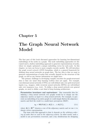
48CHAPTER 5. THE GRAPH NEURAL NETWORK MODELneural networks over graphs is that they should permutation invariant (orequivariant). In mathematical terms, any function f that takes an adjacency matrix A as input should ideally satisfy one of the two followingproperties:f (PAP ) f (A) f (PAP ) Pf (A)(Permutation Invariance)(5.2)(Permutation Equivariance),(5.3)where P is a permutation matrix. Permutation invariance means that thefunction does not depend on the arbitrary ordering of the rows/columns inthe adjacency matrix, while permutation equivariance means that the output of f is permuted in an consistent way when we permute the adjacencymatrix. (The shallow encoders we discussed in Part I are an example ofpermutation equivariant functions.) Ensuring invariance or equivariance isa key challenge when we are learning over graphs, and we will revisit issuessurrounding permutation equivariance and invariance often in the ensuingchapters.5.1Neural Message PassingThe basic graph neural network (GNN) model can be motivated in a variety ofways. The same fundamental GNN model has been derived as a generalizationof convolutions to non-Euclidean data [Bruna et al., 2014], as a di erentiablevariant of belief propagation [Dai et al., 2016], as well as by analogy to classicgraph isomorphism tests [Hamilton et al., 2017b]. Regardless of the motivation,the defining feature of a GNN is that it uses a form of neural message passing inwhich vector messages are exchanged between nodes and updated using neuralnetworks [Gilmer et al., 2017].In the rest of this chapter, we will detail the foundations of this neuralmessage passing framework. We will focus on the message passing frameworkitself and defer discussions of training and optimizing GNN models to Chapter 6.The bulk of this chapter will describe how we can take an input graph G (V, E),along with a set of node features X 2 Rd V , and use this information togenerate node embeddings zu , 8u 2 V. However, we will also discuss how theGNN framework can be used to generate embeddings for subgraphs and entiregraphs.5.1.1Overview of the Message Passing Framework(k)During each message-passing iteration in a GNN, a hidden embedding hu corresponding to each node u 2 V is updated according to information aggregatedfrom u’s graph neighborhood N (u) (Figure 5.1). This message-passing update
5.1. NEURAL MESSAGE PASSING49ATARGET NODEBCBAACAFBaggregateCEDFEDAINPUT GRAPHFigure 5.1: Overview of how a single node aggregates messages from its localneighborhood. The model aggregates messages from A’s local graph neighbors(i.e., B, C, and D), and in turn, the messages coming from these neighbors arebased on information aggregated from their respective neighborhoods, and so on.This visualization shows a two-layer version of a message-passing model. Noticethat the computation graph of the GNN forms a tree structure by unfolding theneighborhood around the target node.can be expressed as follows: (k)(k)(k)(k)h(k 1) UPDATEh,AGGREGATE({h,8v2N(u)})uuv (k) UPDATE(k) h(k)u , mN (u) ,(5.4)(5.5)where UPDATE and AGGREGATE are arbitrary di erentiable functions (i.e., neural networks) and mN (u) is the “message” that is aggregated from u’s graphneighborhood N (u). We use superscripts to distinguish the embeddings andfunctions at di erent iterations of message passing.1At each iteration k of the GNN, the AGGREGATE function takes as input theset of embeddings of the nodes in u’s graph neighborhood N (u) and generates(k)a message mN (u) based on this aggregated neighborhood information. The(k)update function UPDATE then combines the message mN (u) with the previous(k 1)(k)embedding huof node u to generate the updated embedding hu . Theinitial embeddings at k 0 are set to the input features for all the nodes, i.e.,(0)hu xu , 8u 2 V. After running K iterations of the GNN message passing, wecan use the output of the final layer to define the embeddings for each node,i.e.,zu h(K)u , 8u 2 V.(5.6)Note that since the AGGREGATE function takes a set as input, GNNs defined inthis way are permutation equivariant by design.1 The di erent iterations of message passing are also sometimes known as the di erent“layers” of the GNN.
50CHAPTER 5. THE GRAPH NEURAL NETWORK MODELNode features Note that unlike the shallow embedding methods discussed in Part I of this book, the GNN framework requires that we havenode features xu , 8u 2 V as input to the model. In many graphs, we willhave rich node features to use (e.g., gene expression features in biologicalnetworks or text features in social networks). However, in cases where nonode features are available, there are still several options. One option isto use node statistics—such as those introduced in Section 2.1—to definefeatures. Another popular approach is to use identity features, where we associate each node with a one-hot indicator feature, which uniquely identifiesthat node.aa Note, however, that the using identity features makes the model transductive andincapable of generalizing to unseen nodes.5.1.2Motivations and IntuitionsThe basic intuition behind the GNN message-passing framework is straightforward: at each iteration, every node aggregates information from its localneighborhood, and as these iterations progress each node embedding containsmore and more information from further reaches of the graph. To be precise:after the first iteration (k 1), every node embedding contains informationfrom its 1-hop neighborhood, i.e., every node embedding contains informationabout the features of its immediate graph neighbors, which can be reached bya path of length 1 in the graph; after the second iteration (k 2) every nodeembedding contains information from its 2-hop neighborhood; and in general,after k iterations every node embedding contains information about its k-hopneighborhood.But what kind of “information” do these node embeddings actually encode?Generally, this information comes in two forms. On the one hand there is structural information about the graph. For example, after k iterations of GNN(k)message passing, the embedding hu of node u might encode information aboutthe degrees of all the nodes in u’s k-hop neighborhood. This structural information can be useful for many tasks. For instance, when analyzing moleculargraphs, we can use degree information to infer atom types and di erent structural motifs, such as benzene rings.In addition to structural information, the other key kind of informationcaptured by GNN node embedding is feature-based. After k iterations of GNNmessage passing, the embeddings for each node also encode information aboutall the features in their k-hop neighborhood. This local feature-aggregationbehaviour of GNNs is analogous to the behavior of the convolutional kernelsin convolutional neural networks (CNNs). However, whereas CNNs aggregatefeature information from spatially-defined patches in an image, GNNs aggregateinformation based on local graph neighborhoods. We will explore the connectionbetween GNNs and convolutions in more detail in Chapter 7.
5.1. NEURAL MESSAGE PASSING5.1.351The Basic GNNSo far, we have discussed the GNN framework in a relatively abstract fashion asa series of message-passing iterations using UPDATE and AGGREGATE functions(Equation 5.4). In order to translate the abstract GNN framework definedin Equation (5.4) into something we can implement, we must give concreteinstantiations to these UPDATE and AGGREGATE functions. We begin here withthe most basic GNN framework, which is a simplification of the original GNNmodels proposed by Merkwirth and Lengauer [2005] and Scarselli et al. [2009].The basic GNN message passing is defined ash(k)u (k)01)@W(k) h(kself u(k)(k)(k (k)WneighXv2N (u)h(kv1)1 b(k) A ,(5.7)1)where Wself , Wneigh 2 Rd dare trainable parameter matrices anddenotes an elementwise non-linearity (e.g., a tanh or ReLU). The bias term(k)b(k) 2 Rd is often omitted for notational simplicity, but including the biasterm can be important to achieve strong performance. In this equation—andthroughout the remainder of the book—we use superscripts to di erentiate parameters, embeddings, and dimensionalities in di erent layers of the GNN.The message passing in the basic GNN framework is analogous to a standardmulti-layer perceptron (MLP) or Elman-style recurrent neural network, i.e., Elman RNN [Elman, 1990], as it relies on linear operations followed by a singleelementwise non-linearity. We first sum the messages incoming from the neighbors; then, we combine the neighborhood information with the node’s previousembedding using a linear combination; and finally, we apply an elementwisenon-linearity.We can equivalently define the basic GNN through the UPDATE and AGGREGATEfunctions:mN (u) Xhv ,(5.8)v2N (u)UPDATE (hu , mN (u) ) Wself hu Wneigh mN (u) ,(5.9)where we recall that we usemN (u) AGGREGATE(k) ({h(k)v , 8v 2 N (u)})(5.10)as a shorthand to denote the message that has been aggregated from u’s graphneighborhood. Note also that we omitted the superscript denoting the iterationin the above equations, which we will often do for notational brevity.22 In general, the parameters Wself , Wneigh and b can be shared across the GNN messagepassing iterations or trained separately for each layer.
52CHAPTER 5. THE GRAPH NEURAL NETWORK MODELNode vs. graph-level equations In the description of the basic GNNmodel above, we defined the core message-passing operations at the nodelevel. We will use this convention for the bulk of this chapter and this bookas a whole. However, it is important to note that many GNNs can also besuccinctly defined using graph-level equations. In the case of a basic GNN,we can write the graph-level definition of the model as follows: (k)(k)H(t) AH(k 1) Wneigh H(k 1) Wself ,(5.11)where H(k) 2 R V d denotes the matrix of node representations at layer tin the GNN (with each node corresponding to a row in the matrix), A is thegraph adjacency matrix, and we have omitted the bias term for notationalsimplicity. While this graph-level representation is not easily applicable toall GNN models—such as the attention-based models we discuss below—itis often more succinct and also highlights how many GNNs can be efficientlyimplemented using a small number of sparse matrix operations.5.1.4Message Passing with Self-loopsAs a simplification of the neural message passing approach, it is common to addself-loops to the input graph and omit the explicit update step. In this approachwe define the message passing simply as(kh(k)u AGGREGATE ({hv1), 8v 2 N (u) [ {u}}),(5.12)where now the aggregation is taken over the set N (u) [ {u}, i.e., the node’sneighbors as well as the node itself. The benefit of this approach is that weno longer need to define an explicit update function, as the update is implicitlydefined through the aggregation method. Simplifying the message passing in thisway can often alleviate overfitting, but it also severely limits the expressivityof the GNN, as the information coming from the node’s neighbours cannot bedi erentiated from the information from the node itself.In the case of the basic GNN, adding self-loops is equivalent to sharingparameters between the Wself and Wneigh matrices, which gives the followinggraph-level update: H(t) (A I)H(t 1) W(t) .(5.13)In the following chapters we will refer to this as the self-loop GNN approach.5.2Generalized Neighborhood AggregationThe basic GNN model outlined in Equation (5.7) can achieve strong performance, and its theoretical capacity is well-understood (see Chapter 7). However,
5.2. GENERALIZED NEIGHBORHOOD AGGREGATION53just like a simple MLP or Elman RNN, the basic GNN can be improved uponand generalized in many ways. Here, we discuss how the AGGREGATE operatorcan be generalized and improved upon, with the following section (Section 5.3)providing an analogous discussion for the UPDATE operation.5.2.1Neighborhood NormalizationThe most basic neighborhood aggregation operation (Equation 5.8) simply takesthe sum of the neighbor embeddings. One issue with this approach is that it canbe unstable and highly sensitive to node degrees. For instance, suppose nodeu has 100 as many neighbors as Pnode u0 (i.e., a muchP higher degree), thenwe would reasonably expect that k v2N (u) hv k k v0 2N (u0 ) hv0 k (for anyreasonable vector norm k · k). This drastic di erence in magnitude can lead tonumerical instabilities as well as difficulties for optimization.One solution to this problem is to simply normalize the aggregation operationbased upon the degrees of the nodes involved. The simplest approach is to justtake an average rather than sum:Pv2N (u) hvmN (u) ,(5.14) N (u) but researchers have also found success with other normalization factors, such asthe following symmetric normalization employed by Kipf and Welling [2016a]:mN (u) Xhvp. N(u) N(v) v2N (u)(5.15)For example, in a citation graph—the kind of data that Kipf and Welling [2016a]analyzed—information from very high-degree nodes (i.e., papers that are citedmany times) may not be very useful for inferring community membership in thegraph, since these papers can be cited thousands of times across diverse subfields. Symmetric normalization can also be motivated based on spectral graphtheory. In particular, combining the symmetric-normalized aggregation (Equation 5.15) along with the basic GNN update function (Equation 5.9) results ina first-order approximation of a spectral graph convolution, and we expand onthis connection in Chapter 7.Graph convolutional networks (GCNs)One of the most popular baseline graph neural network models—the graphconvolutional network (GCN)—employs the symmetric-normalized aggregationas well as the self-loop update approach. The GCN model thus defines themessage passing function as01Xhv@W(k)A.ph(k)(5.16)u N(u) N(v) v2N (u)[{u}
54CHAPTER 5. THE GRAPH NEURAL NETWORK MODELThis approach was first outlined by Kipf and Welling [2016a] and has proved tobe one of the most popular and e ective baseline GNN architectures.To normalize or not to normalize? Proper normalization can be essential to achieve stable and strong performance when using a GNN. Itis important to note, however, that normalization can also lead to a lossof information. For example, after normalization, it can be hard (or evenimpossible) to use the learned embeddings to distinguish between nodesof di erent degrees, and various other structural graph features can beobscured by normalization. In fact, a basic GNN using the normalized aggregation operator in Equation (5.14) is provably less powerful than thebasic sum aggregator in Equation (5.8) (see Chapter 7). The use of normalization is thus an application-specific question. Usually, normalizationis most helpful in tasks where node feature information is far more usefulthan structural information, or where there is a very wide range of nodedegrees that can lead to instabilities during optimization.5.2.2Set AggregatorsNeighborhood normalization can be a useful tool to improve GNN performance,but can we do more to improve the AGGREGATE operator? Is there perhapssomething more sophisticated than just summing over the neighbor embeddings?The neighborhood aggregation operation is fundamentally a set function.We are given a set of neighbor embeddings {hv , 8v 2 N (u)} and must map thisset to a single vector mN (u) . The fact that {hv , 8v 2 N (u)} is a set is in factquite important: there is no natural ordering of a nodes’ neighbors, and anyaggregation function we define must thus be permutation invariant.Set poolingOne principled approach to define an aggregation function is based on the theoryof permutation invariant neural networks. For example, Zaheer et al. [2017] showthat an aggregation function with the following form is a universal set functionapproximator:01XmN (u) MLP @MLP (hv )A ,(5.17)v2N (u)where as usual we use MLP to denote an arbitrarily deep multi-layer perceptronparameterized by some trainable parameters . In other words, the theoreticalresults in Zaheer et al. [2017] show that any permutation-invariant functionthat maps a set of embeddings to a single embedding can be approximated toan arbitrary accuracy by a model following Equation (5.17).Note that the theory presented in Zaheer et al. [2017] employs a sum of theembeddings after applying the first MLP (as in Equation 5.17). However, it ispossible to replace the sum with an alternative reduction function, such as an
5.2. GENERALIZED NEIGHBORHOOD AGGREGATION55element-wise maximum or minimum, as in Qi et al. [2017], and it is also commonto combine models based on Equation (5.17) with the normalization approachesdiscussed in Section 5.2.1, as in the GraphSAGE-pool approach [Hamilton et al.,2017b].Set pooling approaches based on Equation (5.17) often lead to small increasesin performance, though they also introduce an increased risk of overfitting,depending on the depth of the MLPs used. If set pooling is used, it is common touse MLPs that have only a single hidden layer, since these models are sufficientto satisfy the theory, but are not so overparameterized so as to risk catastrophicoverfitting.Janossy poolingSet pooling approaches to neighborhood aggregation essentially just add extralayers of MLPs on top of the more basic aggregation architectures discussedin Section 5.1.3. This idea is simple, but is known to increase the theoreticalcapacity of GNNs. However, there is another alternative approach, termedJanossy pooling, that is also provably more powerful than simply taking a sumor mean of the neighbor embeddings [Murphy et al., 2018].Recall that the challenge of neighborhood aggregation is that we must usea permutation-invariant function, since there is no natural ordering of a node’sneighbors. In the set pooling approach (Equation 5.17), we achieved this permutation invariance by relying on a sum, mean, or element-wise max to reduce theset of embeddings to a single vector. We made the model more powerful by combining this reduction with feed-forward neural networks (i.e., MLPs). Janossypooling employs a di erent approach entirely: instead of using a permutationinvariant reduction (e.g., a sum or mean), we apply a permutation-sensitivefunction and average the result over many possible permutations.Let i 2 denote a permutation function that maps the set {hv , 8v 2 N (u)}to a specific sequence (hv1 , hv2 , ., hv N (u) ) i . In other words, i takes theunordered set of neighbor embeddings and places these embeddings in a sequencebased on some arbitrary ordering. The Janossy pooling approach then performsneighborhood aggregation by!1 XmN (u) MLP hv1 , hv2 , ., hv N (u) ,(5.18)i 2 where denotes a set of permutations and is a permutation-sensitive function, e.g., a neural network that operates on sequences. In practice is usuallydefined to be an LSTM [Hochreiter and Schmidhuber, 1997], since LSTMs areknown to be a powerful neural network architecture for sequences.If the set of permutations in Equation (5.18) is equal to all possible permutations, then the aggregator in Equation (5.18) is also a universal functionapproximator for sets, like Equation (5.17). However, summing over all possible permutations is generally intractable. Thus, in practice, Janossy poolingemploys one of two approaches:
56CHAPTER 5. THE GRAPH NEURAL NETWORK MODEL1. Sample a random subset of possible permutations during each applicationof the aggregator, and only sum over that random subset.2. Employ a canonical ordering of the nodes in the neighborhood set; e.g.,order the nodes in descending order according to their degree, with tiesbroken randomly.Murphy et al. [2018] include a detailed discussion and empirical comparison ofthese two approaches, as well as other approximation techniques (e.g., truncating the length of sequence), and their results indicate that Janossy-style poolingcan improve upon set pooling in a number of synthetic evaluation setups.5.2.3Neighborhood AttentionIn addition to more general forms of set aggregation, a popular strategy forimproving the aggregation layer in GNNs is to apply attention [Bahdanau et al.,2015]. The basic idea is to assign an attention weight or importance to eachneighbor, which is used to weigh this neighbor’s influence during the aggregationstep. The first GNN model to apply this style of attention was Veličković et al.[2018]’s Graph Attention Network (GAT), which uses attention weights to definea weighted sum of the neighbors:XmN (u) u,v hv ,(5.19)v2N (u)where u,v denotes the attention on neighbor v 2 N (u) when we are aggregatinginformation at node u. In the original GAT paper, the attention weights aredefined asexp a [Whu Whv ] u,v P,(5.20) Whv0 ])v 0 2N (u) exp (a [Whuwhere a is a trainable attention vector, W is a trainable matrix, and denotesthe concatenation operation.The GAT-style attention computation is known to work well with graphdata. However, in principle any standard attention model from the deep learningliterature at large can be used [Bahdanau et al., 2015]. Popular variants ofattention include the bilinear attention model u,v Pexp h u Whv, 0v 0 2N (u) exp (hu Whv )(5.21)as well as variations of attention layers using MLPs, e.g., u,v Pexp (MLP(hu , hv )),exp (MLP(hu , hv0 ))(5.22)v 0 2N (u)where the MLP is restricted to a scalar output.In addition, while it is less common in the GNN literature, it is also possible to add multiple attention “heads”, in the style of the popular transformer
5.2. GENERALIZED NEIGHBORHOOD AGGREGATION57architecture [Vaswani et al., 2017]. In this approach, one computes K distinctattention weights u,v,k , using independently parameterized attention layers.The messages aggregated using the di erent attention weights are then transformed and combined in the aggregation step, usually with a linear projectionfollowed by a concatenation operation, e.g.,mN (u) [a1ak W ka2 . aK ]X u,v,k hv(5.23)(5.24)v2N (u)where the attention weights u,v,k for each of the K attention heads can becomputed using any of the above attention mechanisms.Graph attention and transformers GNN models with multi-headedattention (Equation 5.23) are closely related to the transformer architecture[Vaswani et al., 2017]. Transformers are a popular architecture for bothnatural language processing (NLP) and computer vision, and—in the caseof NLP—they have been an important driver behind large state-of-the-artNLP systems, such as BERT [Devlin et al., 2018] and XLNet [Yang et al.,2019]. The basic idea behind transformers is to define neural network layersentirely based on the attention operation. At each layer in a transformer,a new hidden representation is generated for every position in the inputdata (e.g., every word in a sentence) by using multiple attention heads tocompute attention weights between all pairs of positions in the input, whichare then aggregated with weighted sums based on these attention weights(in a manner analogous to Equation 5.23). In fact, the basic transformerlayer is exactly equivalent to a GNN layer using multi-headed attention(i.e., Equation 5.23) if we assume that the GNN receives a fully-connectedgraph as input.This connection between GNNs and transformers has been exploited innumerous works. For example, one implementation strategy for designingGNNs is to simply start with a transformer model and then apply a binary adjacency mask on the attention layer to ensure that information isonly aggregated between nodes that are actually connected in the graph.This style of GNN implementation can benefit from the numerous wellengineered libraries for transformer architectures that exist. However, adownside of this approach, is that transformers must compute the pairwise attention between all positions/nodes in the input, which leads to aquadratic O( V 2 ) time complexity to aggregate messages for all nodes inthe graph, compared to a O( V E ) time complexity for a more standardGNN implementation.Adding attention is a useful strategy for increasing the representational capacity of a GNN model, especially in cases where you have prior knowledgeto indicate that some neighbors might be more informative than others. Forexample, consider the case of classifying papers into topical categories based
58CHAPTER 5. THE GRAPH NEURAL NETWORK MODELon citation networks. Often there are papers that span topical boundaries, orthat are highly cited across various di erent fields. Ideally, an attention-basedGNN would learn to ignore these papers in the neural message passing, as suchpromiscuous neighbors would likely be uninformative when trying to identifythe topical category of a particular node. In Chapter 7, we will discuss howattention can influence the inductive bias of GNNs from a signal processingperspective.5.3Generalized Update MethodsThe AGGREGATE operator in GNN models has generally received the most attention from researchers—in terms of proposing novel architectures and variations.This was especially the case after the introduction of the GraphSAGE framework,which introduced the idea of generalized neighbourhood aggregation [Hamiltonet al., 2017b]. However, GNN message passing involves two key steps: aggregation and updating, and in many ways the UPDATE operator plays an equallyimportant role in defining the power and inductive bias of the GNN model.So far, we have seen the basic GNN approach—where the update operationinvolves a linear combination of the node’s current embedding with the messagefrom its neighbors—as well as the self-loop approach, which simply involvesadding a self-loop to the graph before performing neighborhood aggregation. Inthis section, we turn our attention to more diverse generalizations of the UPDATEoperator.Over-smoothing and neighbourhood influence One common issuewith GNNs—which generalized update methods can help to address—isknown as over-smoothing. The essential idea of over-smoothing is that afterseveral iterations of GNN message passing, the representations for all thenodes in the graph can become very similar to one another. This tendency isespecially common in basic GNN models and models that employ the selfloop update approach. Over-smoothing is problematic because it makesit impossible to build deeper GNN models—which leverage longer-termdependencies in the graph—since these deep GNN models tend to justgenerate over-smoothed embeddings.This issue of over-smoothing in GNNs can be formalized by defining the(0)influence of each node’s input feature hu xu on the final layer embedding(K)of all the other nodes in the graph, i.e, hv , 8v 2 V. In particular, for anypair of nodes u and v we can quantify the influence of node u on node vin the GNN by examining the magnitude of the corresponding Jacobianmatrix [Xu et al., 2018]:!(K)@hv IK (u, v) 11,(5.25)(0)@huwhere 1 is a vector of all ones. The IK (u, v) value uses the sum of the
5.3. GENERALIZED UPDATE METHODS59@h(K)entries in the Jacobian matrix v(0) as a measure of how much the initial@huembedding of node u influences the final embedding of node v in the GNN.Given this definition of influence, Xu et al. [2018] prove the following:Theorem 3. For any GNN model using a self-loop update approach andan aggregation function of the formAGGREGATE ({hv , 8v2 N (u) [ {u}}) 1fn ( N (u) [ {u} )Xhv ,v2N (u)[{u}(5.26)where f : R ! R is an arbitrary di erentiable normalization function,we have thatIK (u, v) / pG,K (u v),(5.27)where pG,K (u v) denotes the probability of visiting node v on a length-Krandom walk starting from node u.This theorem is a direct consequence of Theorem 1 in Xu et al. [2018].It states that when we are using a K-layer GCN-style model, the influence of node u and node v is proportional the probability of reaching nodev on a K-step random walk starting from node u. An important consequence of this, however, is that as K ! 1 the influence of every nodeapproaches the stationary distribution of random walks over the graph,meaning that local neighborhood information is lost. Moreover, in manyreal-world graphs—which contain high-degree nodes and resemble so-called“expander” graph
data is that our usual deep learning toolbox does not apply. For example, convolutional neural networks (CNNs) are well-defined only over grid-structured inputs (e.g., images), while recurrent neural networks (RNNs) are well-defined only over sequences (e.g., text). To define a deep neural network over general