Transcription
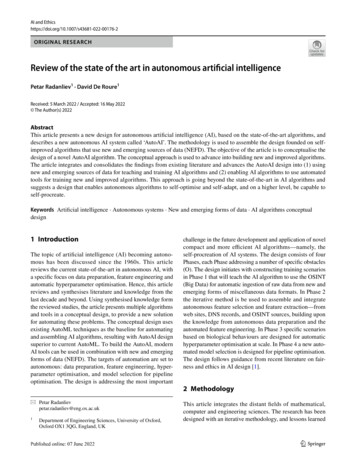
An Autonomous System View To Apply Machine LearningLi-C. WangUniversity of California, Santa BarbaraAbstract—Applying machine learning in design and test hasbeen a growing field of interest in recent years. Many potentialapplications have been demonstrated and tried. This tutorialpaper provides a review of author’s experience in this field, inparticular how the perspective for applying machine learningevolved from one stage to another where the latest perspectiveis based on an autonomous system view to apply machinelearning. The theoretical and practical barriers leading to thisview are highlighted with selected applications.1. IntroductionApplying machine learning in design and test has attracted much interests in recent years. Tremendous amountsof simulation and measurement data are generated andcollected in design and test processes. These data offeropportunities for applying machine learning [1].As a start, applying machine learning could be seen asselecting a tool from a machine learning toolbox (e.g. [2])and running the tool with data collected in an applicationcontext. The goal could be for predicting a behavior in thefuture data, or for understanding the current data at hand.A machine learning tool takes a dataset and produces alearning model. Depending on the underlying algorithm, alearning model, represented in a particular form, might ormight not be interpretable by a person.In many applications, applying machine learning is notjust about choosing a particular tool and obtaining a particular learning model. Often, domain knowledge is required toenable the learning because the data is limited, and applyingmachine learning becomes more like following an iterativesearch process [1]. The focus of the process is on learningabout the features rather than building a model [3].The search process iterates between two agents, an analyst and a toolbox. In each iteration, the analyst decides ananalytic tool to run and the data to run with. The analystprepares the dataset and invokes the tool. The result isthen examined by the analyst to decide what to do next.Figure 1 illustrates this view with the three components:input preparation, tool invocation, and result evaluation.Figure 1. An autonomous system view to apply machine learningIn Figure 1, input preparation and result evaluation arelargely domain knowledge driven. An implication of takingthis view is that in order to automate the search process,all three components need to be automated, resulting in anautonomous system view to apply machine learning.At first glance, Figure 1 seems to suggest that “machinelearning” takes place in the tool invocation box. In otherwords, “applying machine learning” essentially means toinvoke a tool in a machine learning toolbox. If applyingmachine learning means running a machine learning tool,then what the tool is actually learning?Take clustering as an example, which is a commonproblem considered in unsupervised learning. One of thepopular clustering algorithms is K-means [2]. Suppose oneprepares a dataset and runs the K-means tool with thedataset. Suppose k 3, so the output is a partitioning ofthe samples into three groups. If this is “machine learning,”what the K-means tool is learning?Take regression as another example, which is a commonproblem considered in supervised learning. One of the popular regression algorithms is ridge regression. Again, supposeone prepares a dataset and runs the regression tool withthe dataset. Is that “machine learning?” If it is, what is thedifference between “machine learning” and model buildingtaught in a traditional statistics textbook?To define what “machine learning” means in general isbeyond this paper. However, it is important to clarify wheremachine learning takes place in the view of Figure 1. Toanswer that question, an analogy can be drawn betweenFigure 1 and a system view for autonomous vehicle.Figure 2. A system view for autonomous vehicleFigure 2 shows a high-level system view with threecomponents for an autonomous vehicle [4]. The sensingcomponent can be based on a list of sensors such as shortrange radar, long-range radar, LiDAR, ultrasonic, vision,stereo vision, etc. The perception component interprets thedata from those sensors, for example to perform objectrecognition and lane detection, etc. The reasoning and control component calculates the free space for moving the vehicle, plans its path, and controls such as speed/brake/wheel.Paper AI 4.1INTERNATIONAL TEST CONFERENCE978-1-5386-8382-8/18/ 31.00 c 2018 IEEE1
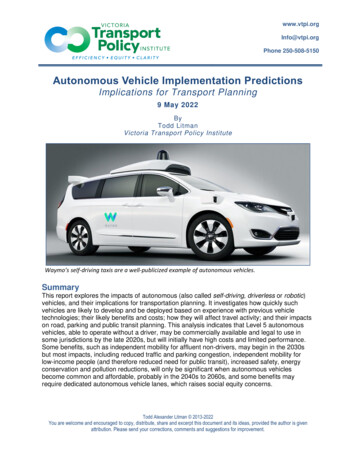
Essentially, the sensing component collects data from theenvironment. The perception component recognizes whatthe data mean. The reasoning and control component decides what to do next. The analogy between Figure 1and Figure 2 is that the tool invocation corresponds tothe sensing component, the result evaluation correspondsto the perception component, and the dataset preparationcorresponds to the reasoning and control component.The analogy might seem unintuitive at first. But it canbecome clear if we consider in Figure 1 where the humanintelligence is involved. In Figure 1, the tool in a toolboxfollows a fixed algorithm. It does not capture the intelligence of a person, in this case the analyst’s. The analyst’sintelligence is involved in the input preparation and resultevaluation. Hence, if we consider “machine learning” as forlearning about human intelligence, then the learning shouldtake place in these two components.Similarly, in Figure 2 the intelligence of a driver isin the perception and reasoning components. The sensingcomponent essentially serves as a mechanical interface tothe real-world environment. In this view, for example it isintuitive to see that a deep neural network can be employedin the perception component, and deep learning [5] is widelyaccepted as a form of machine learning.1.1. Machine learning and AIThe analogy between Figure 1 and Figure 2 becomesclear if one sees “machine learning” as “taking a data-drivenapproach to model human intelligence.” With this interpretation, the link between the tool invocation component and thesensing component is clear, i.e. they both are interfaces tothe environment and they both are not where the analyst’sintelligence is employed. In Figure 2, the environment isthe outside world where the car is driving. In Figure 1, theenvironment can be thought of as the software infrastructureused by the analyst to perform an engineering task.It is important to note that in Figure 1 and Figure 2, machine learning can be applied to model human intelligence inthe left two components, but is not necessary. For example,if the human intelligence can be modeled in terms of a set ofrules, then there might not be a need to take a data-drivenapproach. Based on the views presented in those two figures,suppose the left two components are implemented entirelywith rules. Then such a system can still simulate humanintelligence and hence, can be called an artificial intelligencesystem (e.g. an expert system). However, it does not involvemachine learning and hence, would not be called a machinelearning based system.2. Intelligent Engineering Assistant (IEA)In a more general sense, Figure 1 tries to capture theprocess carried out by a person in performing an engineeringtask. In this sense, the tools involved by the person are notlimited to those tools from a particular machine learningtoolbox. They can include other tools, for example a plottingtool, a data processing tool, etc. Therefore, the autonomousPaper AI 4.1system illustrated in Figure 1 can be thought of as forperforming the task autonomously. Such a system can becalled an Intelligent Engineering Assistant (IEA) [6].As an example, Figure 3 illustrates the scope of anengineering task in the production yield application context.In production, every wafer goes through a sequence oftools (manufacturing equipments). There could be more thanhundreds of tools involved. Data collected in the manufacturing process is organized in three levels [7]. Supposethese data are stored in a production database. After a waferis produced, the test process comprises multiple stages oftesting, including such as class probe (e-test), wafer probe,burn-in, and final test. Suppose data collected in those stagesare stored in a test database.Both databases can be a virtual database and supposethere is an interface to access them. An engineer accessesdata from those databases to perform a task. For example,the task is triggered by observing a potential place toimprove yield, i.e. a yield issue. Then, the engineer usesvarious analytic tools to analyze the data. The aim is touncover some interesting findings [7], such as a correlationbetween an e-test and a type of fails, or a particular patternon a wafer map. The outcome of this analysis is summarizedin a PPT presentation. The engineer brings this presentationto a meeting and discusses possible actions. In Figure 3,input to the autonomous system is the data accessed fromthe interface, and output is a PPT presentation.Figure 3. Tasks performed in the production yield contextIn Figure 3, one can think about the analytics performedby the engineer in terms of a workflow (let it be calledan analytic workflow). It is important to point out thatthis workflow may exist implicitly in the person’s mind,rather than explicitly be written in a document (or capturedby a software script). In essence, building an autonomoussystem is to automate the respective analytic workflow. Thisautomation conceptually is similar to the common practicein a company where a software script is used to automatean established methodology (or flow). The key question is,whether a traditional software script is sufficient to automatethe underlying analytic workflow or not, and if not wheremachine learning can help.INTERNATIONAL TEST CONFERENCE2
2.1. Concept-Based Workflow ProgrammingTo illustrate where machine learning can help, consideran analytic workflow example depicted in Figure 4. Thisworkflow segment is triggered by observing a “yield excursion.” Then, the “low-yield” lots are selected for further analysis. The analysis looks for a “correlation trend”between an e-test and the fails from a test bin. If such a“correlation trend” is found, the fails are used to generatewafer maps and the analysis looks for certain patterns suchas “grid pattern” and “edge failing pattern” on those maps.From this perspective, the paradigm to support buildingan autonomous system in view of Figure 1 can be calledConcept-Based Workflow Programming (CBWP).2.2. Where machine learning is appliedIn view of CBWP, it is then intuitive to see that machinelearning is applied for building a concept recognizer tosupport the workflow programming. Consequently, Figure 3can be re-drawn into a new view as that in Figure 5.In this new view, the workflow is captured in a softwareprogram written in a traditional programming language suchas Python, except that it can make a function call to aconcept recognizer in the concept recognition library. Thelibrary comprises a set of concept recognizers which maybe implemented with a machine learning approach and/or afixed-rule approach. The workflow can also make a call toinvoke a tool in a toolbox which can be a machine learningtoolbox, a plotting toolbox, a data processing toolbox, etc.Figure 4. Illustration of a concept-based workflowIn such a workflow segment, the engineer (or analyst)has a specific perception for what “yield excursion,” “lowyield,” “correlation trend,” “grid pattern,” and “edge failingpattern” mean. Let each of them be called a concept. Toautomate the workflow segment, automatic recognition (ordetermination of the existence) of each concept is needed.Recognition of each concept can be accomplished by writinga software script. However, in some cases it might bechallenging to capture a concept perceived by a person interms of fixed rules. It is for those cases, a data-drivenmachine learning model can become useful [7].Take the concept “correlation trend” as an example. Onecan capture this concept as “having a Pearson correlation 0.8.” With this definition, one can write a software scriptto call the Pearson correlation tool in a toolbox and checkif the correlation coefficient is 0.8 or not. This approachcaptures the concept with a fixed rule.The limitation of using a fixed rule is that it might notcapture the concept entirely as perceived by a person [7].For example, The top plot in the Findings stage of Figure 3shows that as the x value becomes larger, the y value alsodrifts larger. The plot has a x-y correlation coefficient muchsmaller than 0.8, but it has a trend interesting to a person’sperception. Hence, an alternative to recognize the conceptcan be based on a neural network model to capture theperception [7]. A neural network model can be used toenhance the recognition of a particular concept, in additionto using a fixed rule.To enable autonomous execution of a workflow segmentas illustrated in Figure 4, what we need is a library ofconcept recognizers. Conversely, if a library of conceptrecognizers are provided, this library enables the construction of an automatic workflow based on those concepts.Paper AI 4.1Figure 5. Illustration of the three components in an IEA systemIn Figure 5, machine learning is employed to enhancethe capabilities of the workflow. An executable workflowdoes not have to involve any machine learning model.However, the capabilities of such a workflow can be limitedbecause of its limitations for capturing human perception.2.3. Workflow constructionOne may ask the question: Can machine learning beused to learn a workflow model as well? The answer is yes.An earlier work in [8] utilizes process learning to learn aworkflow based on the usage log of analytic tools, whichtracks how an engineer carries out a particular analyticprocess. Learning a workflow can be seen as a form ofknowledge acquisition which can be quite important forapplication contexts where direct construction of a workflowis difficult to practice. Moreover, knowledge acquisitioncan be essential for implementing a scheme to supportknowledge accumulation over time and/or across differentpeople. However, implementing those knowledge acquisition functions adds another layer of complexity to an IEAsystem. If it is not required by the application context, theworkflow in Figure 5 can be constructed manually to speedup the development of the IEA system.In this work, knowledge acquisition is treated as afollow-up work for building an IEA system. A more criticalissue is the availability of the concept recognizers that onedesires to use for constructing a workflow. In view of building a practical IEA system, the development of the conceptrecognition library is more essential than implementing aknowledge acquisition layer.INTERNATIONAL TEST CONFERENCE3
3. Evolution To IEAThe IEA system view in Figure 5 is an intuitive way tothink about where to apply machine learning. Each conceptprovides a functional specification for what is supposed tobe accomplished. The applicability of a machine learningtechnique and a learning model can therefore be assessed interms of the functional specification. Moreover, the goodness of a concept recognizer can be evaluated in the contextof the workflow, i.e. the workflow context provides a way todefine the requirements for a recognizer such as its accuracyand robustness. Without a workflow the added value ofemploying a learning model in practice can be unclear andconsequently, justification for “applying machine learning”can become somewhat debatable.In retrospect, the IEA system view is rather intuitive.However, along the research path leading to this view, itwas not always the case. From the original motivation of“applying machine learning in design and test” to the currentIEA view, the research path actually went through multiplestages where the perspective for applying machine learningevolved from one stage to another.Along the path, a change of perspective often took placeafter realizing the difficulty to overcome a theoretical challenge, a practical constraint, or both, and such realizationwas often triggered after a better understanding of somekey questions (not necessarily after finding a clear answer,because for some questions finding those answers could alsobe hard). These questions include such as: When can we say that a machine has learned?Does the No-Free-Lunch theorem [9] matter?Why cross-validation is needed?How to interpret overfitting?Why the Occam’s Razor principle does not work?Can machine learn with “small” data?When can we call it a machine learning solution?What is the added value of employing such a solution in practice?It is interesting to note that the list misses the obviousquestion: What is the best machine learning algorithm touse? This is because this algorithmic question did not drivethe change of a perspective along the research path.In the rest of the paper, let the discussion start with thefirst question: When can we say that a machine has learned?4. The Theoretical QuestionsTake supervised learning as an example. Figure 6 illustrates a theoretical setup for supervised learning whererelative issues regarding the meaning of “learning” can beexplained. Note that this explanation is for highlightingsome important issues from a practitioner’s perspective andin no way, trying to be mathematically rigorous. In thissetup, there are five areas to make an assumption in order toensure learning. These five areas are labeled in the figure.First, there is the hypothesis space H . H is a set offunctions (hypotheses) and one of them f is the true answerPaper AI 4.1Figure 6. Five areas of assumptions for supervised learningto be learned. Of course this function f is unknown to thelearner. Further, H is also unknown so one needs to makean assumption regarding H . Once assumed, the learningalgorithm operates based on this assumed H .To learn, it is assumed that a sample generator Gproduces a set of m samples x1 , . . . , xm according to anunknown but fixed distribution D. For each sample xi , itslabel yi is given, as calculated by f ( xi ). Then, the datasetcomprising the m pairs ( xi , yi ), is provided to the learner.The learner employs a learning algorithm L to learn. Thealgorithm L outputs its answer h. Ideally, if the answer iscorrect, we would have x generated from G, f ( x) h( x).In theory, f has to be learnable [10][11][12] in orderfor a learning algorithm to achieve some sort of learning.To ensure learnability, assumptions need to be made in viewof the setup, and there are five areas to make an assumption.The first assumption concerns the hypothesis space H .It is intuitive to think that learnability depends on thecomplexity of the assumed H (call it HL to differentiateit from the original unknown H ), i.e. the more complexthe HL is, the more difficult the learning is. However, toformally articulate this intuition, one needs a formal way todefine what “complexity” means.If HL is finite and enumerable, then its complexity canbe measured more easily. For example, if HL is the setof all Booleanfunctions based on n variables, then HLncontains 22 distinct functions.Hence, its complexity cannbe characterized as O(22 ), i.e. its size.The difficulty is when the assumed HL is not restrictedto be finite and enumerable, i.e. it can be infinite and/oruncountable. In this case, one cannot rely on counting to sayabout its complexity. One theory to measure the complexityof an assumed HL is based on its ability to fit the data. Thisconcept is called capacity of the hypothesis space which canbe characterized in terms of the VC dimension [12].The VC dimension (VC-D) also represents the minimumnumber of samples required to identify a f randomly chosenfrom HL . Therefore, in order to ensure learning one needs tomake an assumption on the VC-D, for example VC-D shouldbe on the order of poly(n) (polynomial in n, the numberof features). Otherwise, the number of required samples canbe too large for the learning to be practical.The second assumption concerns the sample generatorG. The common assumption is that G produces its samplesby drawing a sample randomly according to a fixed distribution D. Hence, as far as the learning concerns, all futuresamples are generated according to the same distribution D.The third assumption concerns the number of samples(m) available to the learning algorithm. This m has to be atINTERNATIONAL TEST CONFERENCE4
least as large as the VC-D. Otherwise, the samples are notenough for learning the answer f .Even though the samples are sufficient (because weassume the samples are generated randomly, this is thesame as saying that m is sufficiently large), we still need toconcern if there exists a computationally efficient learningalgorithm L to learn it. In most cases, learning the functionf can be computationally hard [11].The computational hardness can be characterized interms of the traditional NP-Hardness notion [11] or thehardness for breaking a cryptography function [13]. Forexample, learning a 3-term DNF (Disjunctive Normal Form)formula using the DNF representation is hard [11]. In fact,except for a few special cases, learning based on a Booleanfunctional class is usually hard [11]. Moreover, learningbased on a simple neural network is hard [14]. The computational hardness implies that in practice for most of theinteresting learning problems, the learning algorithm canonly be a heuristic. Consequently, its performance cannotbe guaranteed for all problem instances.The last assumption concerns how the answer h isevaluated. In the discussion of the other assumed areasabove, we implicitly assume that the ”closeness” of h tof is evaluated through an error function Err(), for exampleErr(h, f ) P rob(h( x) 6 f ( x)) for a randomly drawn x.Notice that with such an Err(), an acceptable answer doesnot require h f . As far as the learning concerns, as longas their outputs are the same with a high probability, h canbe an acceptable answer for f .Such an error function is widely acceptable because inmost of the applications the purpose of the learning is forprediction and the goal is to have a predictor whose accuracyis high enough. However, for applications in design andtest such a view for evaluating the learning result can bemisleading, for example when the use of a learning modelis not for prediction, but for interpretation.To see the intuition, consider that f is the AND functionof 100 Boolean variables, i.e. f ( x) x1 x2 · · · x100 . Fora randomly generated input x, it is almost for sure thatf ( x) 0. As a result, for a given set of m samples itis likely that all we see in the dataset is that y 0.The learner would output the hypothesis “h 0” as theanswer. How good is this answer? From the error functionperspective, this answer is very accurate because the probability, P rob(h( x) 6 f ( x)) for a randomly drawn x, is very1. On the other hand,small, i.e. the probability is only 2100“h 0” is certainly not the correct answer and perhapsnot a desirable answer in practice. In fact, the example f iscalled a “needle-in-a-haystack” function and the No-FreeLunch [9] holds for learning such a function [15] (based onthe demand to find the exact answer).4.1. Learning can be hard in practiceIn theory, learning is hard [15]. In practice, learning canbe even harder. For a practitioner, the first challenge faced isto make a proper assumption regarding the hypothesis spaceH to begin with. This assumption essentially limits what fPaper AI 4.1could be learned from the data. In most of the practicalcases, there is no way to know if an assumed HL is properor not. Hence, in most cases the approach is to make anassumption that is as conservative as possible, for exampleto assume a HL whose capacity is as large as possible.However, in practice the capacity of the assumed HL isalso constrained by two other factors, the data availabilityand the computational power to execute the learning algorithm. If HL is too complex, one might not have sufficientdata to learn about f . Even with sufficient data, one mightnot have the computational resource to run the learning algorithm that can get to f . For example, this second constraintcan be observed in the recent trend of hardware accelerationfor deep learning neural networks [5].The second challenge is that it is difficult to know ifthe data is sufficient. In theory the capacity of an assumedHL can be measured in terms of its VC dimension [12]. Inpractice the effective capacity of a hypothesis space is alsolimited by the learning algorithm [5], making its estimationquite difficult. Consequently, unless the assumed HL issimple enough to allow enumeration of all its hypotheses, itscapacity is usually unknown, making it difficult to determineif the data is sufficient or not.The third challenge comes from the learning algorithm.As mentioned above, a learning algorithm is likely to bejust a heuristic. Its performance is not guaranteed. Also, thebehavior of an algorithm can be parametrized and choosingthe parameter values can further add to the challenge.On top of all these challenges, it is also difficult to ensurethat the generator indeed follows the same fixed distributionin the future when a learning model is applied.4.2. Learning theories and the No-Free-LunchWhen can we say that a machine has learned? Answering the question can be quite challenging. One one hand,there are four theoretical frameworks trying to answer thequestion in supervised learning: the PAC (Probably Approximately Correct) [10][11] framework, the VC framework(the Statistical Learning Theory) [12], the SP framework(the Statistical Physics) (e.g. see [16]), and the Bayesianframework (e.g. see [17]). On the other hand, there is theNo-Free-Lunch (NFL) theorem for learning [9] and NFLholds even in view of the four learning frameworks [18].As discussed in [18], the main reason why none of thefour frameworks can prove learning is because in order todo so, one has to allow all of the four things to vary (incontrast to fixing or discard any of them) in the formalism.These four things are, the hypothesis space H (and the f ),the data, the the assumed HL (and the h), and the costmeasuring the goodness of h for f . In view of [18], themost general framework among the four is the Bayesianframework. However, it does not explicitly separate theassumed HL from the unknown H in the formalism.On the surface, NFL says that in general there is nolearning, if learning means to learn from the samples at handto predict about the unseen samples. More specifically, thereis no one learning algorithm whose performance on averageINTERNATIONAL TEST CONFERENCE5
is better than another, i.e. no algorithm is better than randomguessing (and hence no learning). In view of Figure 6, onecan think that NFL holds in general when one fails to justifythe assumption made on H . Moreover, a variant of NFLholds if H satisfies a certain property [19].In practice, practitioners often dismiss NFL based onthe thinking that in a real world problem the H to belearned on cannot include all possible functions. To see this,assume that H is the set of all Booleanfunctions based onnn variables. The size of H is 22 . However, implementingmost of these functions requires a circuit of O(2n ) sizewhich are unlikely to exist in the real world.Such a thinking might have a point. However, it alsopoints out that there is a need for making a realistic assumption regarding H . Once a practitioner makes an assumptionon H to avoid NFL, how does one know the assumption isindeed realistic? This is a fundamental question that makesanswering the original question hard.4.3. NFL in practiceTo illustrate an intuition behind NFL, consider the simple setup in Figure 7. Suppose the generator G produces thesamples to cover 7 points in the Boolean space based onthe three variables x1 , x2 , x3 . The learning might be seenas uncovering the true Boolean function that governs theinput-output relationship.produces the answer: fa0 ( x) 1 if x3 0.5; otherwisefa0 ( x) 0. This model also shows high accuracy, i.e. aboveor about 93.75% on the validation dataset. Is that learningor is that simply minimization plus noise filtering?The simple example illustrates that it might be difficultto claim that a machine has learned in practice. The commoncross-validation approach does not guarantee that. Crossvalidation might be more meaningful if there is no overlapbetween the training dataset and the validation dataset after“noise filtering.” But it can be challenging to draw theboundary between what is “noise” and what is not.5. Machine Learning To A PractitionerWhen applying a machine learning algorithm, a practitioner is often instructed to pay attention to the notion ofoverfitting. In practice, one is often instructed to observeoverfitting in cross-validation. Let DT and DV denote thetraining and validation datasets. Let EmErr(h, D) be anerror function to report an empirical error rate by applyinga model h onto the dataset D. Let the training error ratebe eT EmErr(h, DT ) and validation error rate beeV EmErr(h, DV ). In learning, a learning algorithm hasonly DT to work on. Hence, the algorithm tries to improveon eT without knowing eV .Figure 8. Overfitting Vs. Underfitting (Traditional View)Figure 7. An example to illustrate NFLBecause there is only one unknown sample “110” left,the true answer can be either fa ( x) x3 or fb ( x) x3 x1 x2 x03 , i.e. fa (110) 0 or fb (110) 1. Supposea learning algorithm chooses fa as the answer becauseit is simpler. Then, based on the common error function1mentioned before, we have Err(fa , f ) 16, i.e. at leasta 93.75% accuracy. But is this learning? After all, if fb is1chosen we also have Err(fb , f ) 16.In view of NFL, the error should be based on only theunseen sample 110. Because f (110) can be either 0 or 1and because seeing other samples p
As a start, applying machine learning could be seen as selecting a tool from a machine learning toolbox (e.g. [2]) and running the tool with data collected in an application context. The goal could be for predicting a behavior in the future data, or for understanding the current data at hand. A machine learning tool takes a dataset and produces a