WIXLIB

TargetSchema“sql-dba”“sql-dba” g)ComputeTaskjobcluster(string) (string)“db.server”“db.server” 18323task abaseService” hService”“Insert”“Query”. Schema10:4210:42.10:4210:4210:42. .value columntime series key columnsFigure 2: Monarch data model example. The top left is a target schema named ComputeTask with four key columns.The top right is the schema for a metric named /rpc/server/latency with two key columns and one value column. Eachrow of the bottom table is a time series; its key is the concatenation of all key columns; its value column is named after thelast part of its metric name (i.e., latency). Each value is an array of timestamped value points (i.e., distributions in thisparticular example). We omit the start time timestamps associated with cumulative time series.Monarch components can be divided by function into threecategories: those holding state, those involved in data ingestion, and those involved in query execution.The components responsible for holding state are: Leaves store monitoring data in an in-memory timeseries store. Recovery logs store the same monitoring data as theleaves, but on disk. This data ultimately gets rewritteninto a long-term time series repository (not discusseddue to space constraints). A global configuration server and its zonal mirrorshold configuration data in Spanner [13] databases.The data ingestion components are: Ingestion routers that route data to leaf routers inthe appropriate Monarch zone, using information intime series keys to determine the routing. Leaf routers that accept data to be stored in a zoneand route it to leaves for storage. Range assigners that manage the assignment of datato leaves, to balance the load among leaves in a zone.The components involved in query execution are: Mixers that partition queries into sub-queries thatget routed to and executed by leaves, and merge subquery results. Queries may be issued at the root level(by root mixers) or at the zone level (by zone mixers).Root-level queries involve both root and zone mixers. Index servers that index data for each zone and leaf,and guide distributed query execution. Evaluators that periodically issue standing queries(see Section 5.2) to mixers and write the results backto leaves.Note that leaves are unique in that they support all threefunctions. Also, query execution operates at both the zonaland global levels.3.DATA MODELConceptually, Monarch stores monitoring data as time series in schematized tables. Each table consists of multiplekey columns that form the time series key, and a value column for a history of points of the time series. See Figure 2for an example. Key columns, also referred to as fields, havetwo sources: targets and metrics, defined as follows.3.1TargetsMonarch uses targets to associate each time series with itssource entity (or monitored entity), which is, for example,the process or the VM that generates the time series. Eachtarget represents a monitored entity, and conforms to a target schema that defines an ordered set of target field namesand associated field types. Figure 2 shows a popular targetschema named ComputeTask; each ComputeTask target identifies a running task in a Borg [46] cluster with four fields:user, job, cluster, and task num.For locality, Monarch stores data close to where the datais generated. Each target schema has one field annotatedas location; the value of this location field determines thespecific Monarch zone to which a time series is routed andstored. For example, the location field of ComputeTask iscluster; each Borg cluster is mapped to one (usually theclosest) Monarch zone. As described in Section 5.3, locationfields are also used to optimize query execution.Within each zone, Monarch stores time series of the sametarget together in the same leaf because they originate fromthe same entity and are more likely to be queried togetherin a join. Monarch also groups targets into disjoint targetranges in the form of [Sstart , Send ) where Sstart and Sendare the start and end target strings. A target string represents a target by concatenating the target schema name andfield values in order1 . For example, in Figure 2, the targetstring ComputeTask::sql-dba::db.server::aa::0876 represents the Borg task of a database server. Target ranges areused for lexicographic sharding and load balancing amongleaves (see Section 4.2); this allows more efficient aggregation across adjacent targets in queries (see Section 5.3).1The encoding also preserves the lexicographic order ofthe tuples of target field values, i.e., S(ha1 , a2 , · · · , an i) S(hb1 , b2 , · · · , bn i) ha1 , a2 , · · · , an i hb1 , b2 , · · · , bn i,where S() is the string encoding function, and ai and bi arethe i-th target-field values of targets a and b, respectively.3183

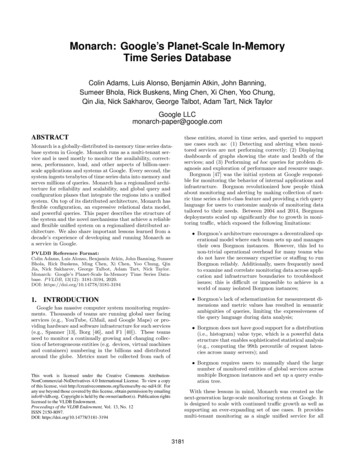
Count20202020101010100000102030010:40 10:41102010:40 10:4230RPC Latency(ms)00102010:40 10:43300102010:43 10:44Figure 3: An example cumulative distribution timeseries for metric /rpc/server/latency. There are fourpoints in this time series; each point value is a histogram,whose bucket size is 10ms. Each point has a timestamp anda start timestamp. For example, the 2nd point says thatbetween 10:40 and 10:42, a total of 30 RPCs were served,among which 20 RPCs took 0–10ms and 10 RPCs took 10–20ms. The 4th point has a new start timestamp; between10:43 and 10:44, 10 RPCs were served and each took 0–10ms.3.2Bucket: [6.45M . 7.74M)Count: 1Exemplar value: 6.92.M@2019/8/16 10:53:27RPC Trace30MetricsA metric measures one aspect of a monitored target, suchas the number of RPCs a task has served, the memory utilization of a VM, etc. Similar to a target, a metric conformsto a metric schema, which defines the time series value typeand a set of metric fields. Metrics are named like files. Figure 2 shows an example metric called /rpc/server/latencythat measures the latency of RPCs to a server; it has twometric fields that distinguish RPCs by service and command.The value type can be boolean, int64, double, string,distribution, or tuple of other types. All of them arestandard types except distribution, which is a compacttype that represents a large number of double values. Adistribution includes a histogram that partitions a set ofdouble values into subsets called buckets and summarizesvalues in each bucket using overall statistics such as mean,count, and standard deviation [28]. Bucket boundaries areconfigurable for trade-off between data granularity (i.e., accuracy) and storage costs: users may specify finer bucketsfor more popular value ranges. Figure 3 shows an example distribution-typed time series of /rpc/server/latencywhich measures servers’ latency in handling RPCs; and ithas a fixed bucket size of 10ms. Distribution-typed pointsof a time series can have different bucket boundaries; interpolation is used in queries that span points with differentbucket boundaries. Distributions are an effective feature forsummarizing a large number of samples. Mean latency is notenough for system monitoring—we also need other statisticssuch as 99th and 99.9th percentiles. To get these efficiently,histogram support—aka distribution—is indispensable.Exemplars. Each bucket in a distribution may containan exemplar of values in that bucket. An exemplar for RPCmetrics, such as /rpc/server/latency, may be a DapperRPC trace [41], which is very useful in debugging high RPClatency. Additionally, an exemplar contains information ofits originating target and metric field values. The information is kept during distribution aggregation, therefore a usercan easily identify problematic tasks via outlier exemplars.Figure 4 shows a heat map of a distribution-typed time series including the exemplar of a slow RPC that may explainthe tail latency spike in the middle of the graph.Metric types. A metric may be a gauge or a cumulative. For each point of a gauge time series, its value isan instantaneous measurement, e.g., queue length, at thetime indicated by the point timestamp. For each point ofa cumulative time series, its value is the accumulation ofthe measured aspect from a start time to the time indicatedExemplar Fieldsuser: Monarchjob: mixer.zone1cluster: aatask num: 0service: MonarchServicecommand: QueryGo to TaskFigure 4: A heat map of /rpc/server/latency. Clicking an exemplar shows the captured RPC trace.by its timestamp. For example, /rpc/server/latency inFigure 3 is a cumulative metric: each point is a latency distribution of all RPCs from its start time, i.e., the start timeof the RPC server. Cumulative metrics are robust in thatthey still make sense if some points are missing, becauseeach point contains all changes of earlier points sharing thesame start time. Cumulative metrics are important to support distributed systems which consist of many servers thatmay be regularly restarted due to job scheduling [46], wherepoints may go missing during restarts.4.SCALABLE COLLECTIONTo ingest a massive volume of time series data in realtime, Monarch uses two divide-and-conquer strategies andone key optimization that aggregates data during collection.4.1Data Collection OverviewThe right side of Figure 1 gives an overview of Monarch’scollection path. The two levels of routers perform two levels of divide-and-conquer: ingestion routers regionalize timeseries data into zones according to location fields, and leafrouters distribute data across leaves according to the rangeassigner. Recall that each time series is associated with atarget and one of the target fields is a location field.Writing time series data into Monarch follows four steps:1. A client sends data to one of the nearby ingestionrouters, which are distributed across all our clusters.Clients usually use our instrumentation library, whichautomatically writes data at the frequency necessaryto fulfill retention policies (see Section 6.2.2).2. The ingestion router finds the destination zone basedon the value of the target’s location field, and forwardsthe data to a leaf router in the destination zone. Thelocation-to-zone mapping is specified in configurationto ingestion routers and can be updated dynamically.3. The leaf router forwards the data to the leaves responsible for the target ranges containing the target.Within each zone, time series are sharded lexicographically by their target strings (see Section 4.2). Each leafrouter maintains a continuously-updated range mapthat maps each target range to three leaf replicas.Note that leaf routers get updates to the range mapfrom leaves instead of the range assigner. Also, targetranges jointly cover the entire string universe; all new3184

targets will be picked up automatically without intervention from the assigner. So data collection continuesto work if the assigner suffers a transient failure.4. Each leaf writes data into its in-memory store and recovery logs. The in-memory time series store is highlyoptimized: it (1) encodes timestamps efficiently andshares timestamp sequences among time series fromthe same target; (2) handles delta and run-length encoding of time series values of complex types includingdistribution and tuple; (3) supports fast read, write,and snapshot; (4) operates continuously while processing queries and moving target ranges; and (5) minimizes memory fragmentation and allocation churn. Toachieve a balance between CPU and memory [22], thein-memory store performs only light compression suchas timestamp sharing and delta encoding. Timestampsharing is quite effective: one timestamp sequence isshared by around ten time series on average.Note that leaves do not wait for acknowledgement whenwriting to the recovery logs per range. Leaves write logs todistributed file system instances (i.e., Colossus [18]) in multiple distinct clusters and independently fail over by probing the health of a log. However, the system needs to continue functioning even when all Colossus instances are unavailable, hence the best-effort nature of the write to thelog. Recovery logs are compacted, rewritten into a formatamenable for fast reads (leaves write to logs in a writeoptimized format), and merged into the long-term repositoryby continuously-running background processes whose detailswe omit from this paper. All log files are also asynchronouslyreplicated across three clusters to increase availability.Data collection by leaves also triggers updates in the zoneand root index servers which are used to constrain queryfanout (see Section 5.4).4.2Intra-zone Load BalancingAs a reminder, a table schema consists of a target schemaand a metric schema. The lexicographic sharding of datain a zone uses only the key columns corresponding to thetarget schema. This greatly reduces ingestion fanout: ina single write message, a target can send one time seriespoint each for hundreds of different metrics; and having allthe time series for a target together means that the writemessage only needs to go to up to three leaf replicas. Thisnot only allows a zone to scale horizontally by adding moreleaf nodes, but also restricts most queries to a small subset ofleaf nodes. Additionally, commonly used intra-target joinson the query path can be pushed down to the leaf-level,which makes queries cheaper and faster (see Section 5.3).In addition, we allow heterogeneous replication policies (1to 3 replicas) for users to trade off between availability andstorage cost. Replicas of each target range have the sameboundaries, but their data size and induced CPU load maydiffer because, for example, one user may retain only the firstreplica at a fine time granularity while another user retainsall three replicas at a coarse granularity. Therefore, therange assigner assigns each target range replica individually.Of course, a leaf is never assigned multiple replicas of a singlerange. Usually, a Monarch zone contains leaves in multiplefailure domains (clusters); the assigner assigns the replicasfor a range to different failure domains.Range assigners balance load in ways similar to Slicer [1].Within each zone, the range assigner splits, merges, andmoves ranges between leaves to cope with changes in theCPU load and memory usage imposed by the range on theleaf that stores it. While range assignment is changing, datacollection works seamlessly by taking advantage of recoverylogs. For example (range splits and merges are similar), thefollowing events occur once the range assigner decided tomove a range, say R, to reduce the load on the source leaf:1. The range assigner selects a destination leaf with lightload and assigns R to it. The destination leaf starts tocollect data for R by informing leaf routers of its newassignment of R, storing time series with keys withinR, and writing recovery logs.2. After waiting for one second for data logged by thesource leaf to reach disks2 , the destination leaf startsto recover older data within R, in reverse chronological order (since newer data is more critical), from therecovery logs.3. Once the destination leaf fully recovers data in R,it notifies the range assigner to unassign R from thesource leaf. The source leaf then stops collecting datafor R and drops the data from its in-memory store.During this process, both the source and destination leavesare collecting, storing, and logging the same data simultaneously to provide continuous data availability for the rangeR. Note that it is the job of leaves, instead of the range assigner, to keep leaf routers updated about range assignmentsfor two reasons: (1) leaves are the source of truth where datais stored; and (2) it allows the system to degrade gracefullyduring a transient range assigner failure.4.3Collection AggregationFor some monitoring scenarios, it is prohibitively expensive to store time series data exactly as written by clients.One example is monitoring disk I/O, served by millions ofdisk servers, where each I/O operation (IOP) is accountedto one of tens of thousands of users in Google. This generates tens of billions of time series, which is very expensiveto store naively. However, one may only care about the aggregate IOPs per user across all disk servers in a cluster.Collection aggregation solves this problem by aggregatingdata during ingestion.Delta time series. We usually recommend clients usecumulative time series for metrics such as disk IOPs becausethey are resilient to missing points (see Section 3.2). However, aggregating cumulative values with very different starttimes is meaningless. Therefore, collection aggregation requires originating targets to write deltas between adjacentcumulative points instead of cumulative points directly. Forexample, each disk server could write to Monarch every TDseconds the per-user IOP counts it served in the past TD seconds. The leaf routers accept the writes and forward all thewrites for a user to the same set of leaf replicas. The deltascan be pre-aggregated in the client and the leaf routers, withfinal aggregation done at the leaves.2Recall that, to withstand file system failures, leaves do notwait for log writes to be acknowledged. The one secondwait length is almost always sufficient in practice. Also,the range assigner waits for the recovery from logs to finishbefore finalizing the range movement.3185

TrueTime.now.latest{ fetch ComputeTask ::/ rpc / server / latency filter user " monarch " align delta (1 h ); fetch ComputeTask ::/ build / label filter user " monarch " && job " mixer .* "} join group by [ label ] , aggregate ( latency )1TWAdmission WindowTBbucket(finalized)The oldest delta is rejectedbecause its end time is outof the admission window.bucket34bucketxdelta256deltaTDdeltaThe two latestdeltas are admittedinto the two latestbuckets.Figure 5: Collection aggregation using buckets anda sliding admission window.7Figure 6: An example query of latency distributionsbroken down by build label. The underlined are tableoperators. delta and aggregate are functions. “ ” denotes regular expression matching.Key column: label (aka /build/label)Bucketing. During collection aggregation, leaves putdeltas into consecutive time buckets according to the endtime of deltas, as illustrated in Figure 5. The bucket lengthTB is the period of the output time series, and can be configured by clients. The bucket boundaries are aligned differently among output time series for load-smearing purposes.Deltas within each bucket are aggregated into one point according to a user-selected reducer; e.g., the disk I/O exampleuses a sum reducer that adds up the number of IOPs for auser from all disk servers.Admission window. In addition, each l

dencies, Monarch stores monitoring data in memory despite the high cost. Most of Google's storage systems, includ-ing Bigtable [10], Colossus ([36], the successor to GFS [20]), Spanner [13], Blobstore [18], and F1 [40], rely on Monarch for reliable monitoring; thus, Monarch cannot use them on the alerting path to avoid a potentially dangerous .