WIXLIB

Importantly, this adaptive refinement occurs not just spatially, buttemporally as well. As the simulation evolves, a regridding algorithmtests and refines grid cells with a frequency directly related to theirlevel of refinement. Thus, grid cells of fine refinement – indicatingregions of complex or important behavior – undergo testing for regridding more frequently than grid cells of comparatively coarser refinement. This adaptive spatial and temporal refining of the domain spaceresults in a hierarchy of nested, sequentially refined grids that are computationally cheaper to construct and are less expensive to store than ahigh-density uniform grid.Though AMR was first presented in 1984 [5], and then extended in1989 [6], the challenges of mapping common visualization techniquesto AMR’s spatially dynamic grid structure were not addressed untilmuch later. One of the earliest examples of AMR visualization wasgiven by Max [20] in his cell-sorting method for volume rendering.Norman et al. [21] convert AMR hierarchies into finite-element hexahedral cells with cell centered data, thus enabling the use of standardvisualization tools.More recent work focuses upon operating directly on AMR data.Work by Ma [19] describes a parallel rendering strategy for AMRdata and presents two contrasting visualization approaches. Weber etal. [27, 29] present software and hardware-accelerated methods basedon cell projection that facilitate direct volume rendering of AMR data.In their work, they render an AMR hierarchy by starting with its coarsest representation. The image is then refined by subsequently integrating the results obtained from renderings of finer grids. Weber etal. [28] also present crack-free isosurface extraction methods for AMRdata. Park et al. [23] present a hierarchical multi-resolution splattingtechnique for AMR data that utilizes kd-trees and octrees. Their novelapproach provides interactive performance for modest sized data.Kähler and Hege [14] present a hardware-accelerated volumerendering approach to visualize AMR data. Their work, based on 3Dtextures, directly utilizes the hierarchical grid structure of the AMRdata to rapidly render high-resolution datasets – including AMR dataconsisting of over nine levels of refinement. Kähler et al. also presenta novel strategy for remotely visualizing AMR data at intermediatetime steps [15]. Their method utilizes so-called “keyframe” timestepsto generate intermediate grid hierarchies. Data for these grid structuresis then acquired through interpolation strategies (via Hermite or linearmethods) by using the existing data in the keyframe timesteps.Kähler et al. have more recently extended their earlier work bypresenting a GPU-assisted raycasting strategy for accelerating the visualization of AMR data [16]. This work utilizes a kd-tree, resident onthe GPU, to provide a view-consistent ordering of data, and accelerate the task of volume rendering. They contrast their method’s resultswith a hardware accelerated slice-based volume rendering approach.Their method generates superior images to the slice-based approach,with no observable artifacts.2.2 Query-Driven VisualizationQuery-Driven Visualization (QDV) is an important and effective wayto combine database and visualization technologies. QDV strategiesare based on the observation that smaller subsets of data are usuallythe genesis of insight or breakthroughs to new trends [3, 11]. In QDV,users begin analysis by forming definitions for data that are “important” to them. This characterization consists of constructing rangeconstraints for variables of interest. As an example, a user analyzing acombustion dataset may set constraints over specific variables such as:(1100 temperature 1800) AND (pressure 780). QDV methodsuse these range constraints to filter data records passed to visualizationand analysis software. This query filtration process focuses visualization and analytical resources exclusively on data that is meaningful tothe user.Stockinger et al. [25] were first to present the notion of couplingvisualization with high performance query technology. Their workdemonstrates that the computational complexity of visualization processing can be constrained to the number of items returned by a query.Their approach introduces a software system (DEX) that utilizes ahighly efficient indexing and query infrastructure, called FastBit, torapidly identify records of interest [32, 33].Gosink et al. [9] extend the utility of QDV methods by using correlation fields to explore variable interactions within the domain spaceof query-regions. Their work focuses on characterizing flame-frontregions in combustion simulations.Bethel et al. apply QDV principles to network traffic analysis [7].They use compressed bitmap indices to visualize and characterize over2.5 billion records of network connection data. Stockinger et al. [24]extend the QDV approach for traffic analysis by presenting a family ofnew parallel algorithms that generate queryable two-dimensional conditional histograms. These conditional histograms are used to detectand characterize distributed scans.2.3 Multitemporal VisualizationThough researchers have proposed various methods to track timevarying features across multiple timesteps in sequential fashion (i.e.animations), less attention has been paid to the direct visualization of4D data. In direct visualization of 4D data, or multitemporal visualization, important features from selected timesteps are conveyed in a single meaningful visualization. Projecting four-dimensional informationmeaningfully onto a two-dimensional image is difficult to do withoutsaturating the visualization with too much information. Finding waysto extend traditional, three-dimensional visualization methods to fourdimensions is one intuitive way to approach visualizing time-varyingdata.Hansen et al. [12,13] use 3D scalar fields as elevation maps in 4D. Inthese works, 4D lighting, shading, and plane-tracing (i.e. 4D ray tracing) are used to visualize higher dimensional data. Bajaj et al. [2] extend object splatting techniques to present a generalized hyper-volumesplatting approach. Their method presents a multi-resolution algorithm for providing insightful visualizations of scalar fields in any dimension; the focus of their work, however, is not explicit temporalfeature tracking. Bhaniramka et al. [8] extend and generalize marching methods to higher dimensions, specifically generating 4D isosurfaces that can be sliced to enable the study of time-evolving features.Woodring et al. [31] also extend slicing techniques for the direct rendering of 4D space-time volumes (as apposed to the 4D isosurfacesgenerated by Bhaniramka’s work). Their hyper-projection method displays unique spatiotemporal features. Woodring and Shen [30] presenta way to directly volume render time-varying data in a single multitemporal image. In their work, they orthographically project fourdimensional data (i.e. volume data accumulated over time) onto a threedimensional image plane. They use traditional rendering methods overthe image plane, using opacity values that are spatially and temporallybased, to realize multitemporal images.Extending AMR and QDV WorkTo date, no techniques exist that facilitate the rendering of timevarying AMR data in a multitemporal fashion. We address this important issue in this work by combining GPU-based QDV methods witha new approach for temporally synchronizing the time-varying datafrom a series of AMR timesteps. The results of our method allow forthe interactive visualization of multivariate, spatiotemporal AMR data.We also extend previous QDV work in two aspects: we present the firstapplication of QDV techniques on AMR data, and we also present thefirst GPU-based QDV approach that utilizes a GPU-based indexingstrategy to accelerate query processing, efficiently utilize GPU memory, and accelerate QDV methods.3 M ETHODQuery-driven analysis and multitemporal visualization of AMR dataare hindered by the dynamic temporal and spatial properties of AMRbased simulations. Specifically, in AMR-based simulations, any fixedspatial location in the domain can be covered by a grid cell of varying refinement based upon the timestep analyzed. For query-drivenvisualization (QDV), this disparity in refinement between timestepsprevents the evaluation of multitemporal queries. Similarly, coherent multitemporal renderings of AMR data from any visualizationapproach – extracting and simultaneously rendering isosurfaces from

multiple timesteps, or volume rendering with time-dependent transferfunctions – also require addressing these temporal-based disparities ofspatial refinement.Our new method addresses these challenges by synchronizing allAMR grid hierarchies (from any subset of timesteps) with a compositetemplate. This synchronization process facilitates query-driven analysis and multitemporal visualization in two aspects: temporally sequential visualizations, where features from these timesteps are analyzed insequential frames as a movie, and temporally concurrent visualizationswhere a single multitemporal image conveys the important featuresfrom all synchronized timesteps.We base our method on the AMR grid hierarchy outlined by Bergerand Colella [5,6]. We outline this hierarchy and its properties next. Formore details regarding AMR-based simulations, we refer the readerto [1, 5, 6].be covered by some G1,b as well as G0,c . With each refinement levelpossessing a different set of data for the specific region, a visualizationmethod can take one of several approaches to utilize this data [18]:3.1 AMR Grid StructureAdaptive mesh refinement (AMR) implementations are traditionallybased on a nested hierarchy of successively refined axis-aligned grids.These grids are identified using the notation Gl,k where l indicates thelevel of cell refinement for the grid, and k is the unique number forthe grid given this refinement level [6]. We use the notation Gl,k k nto refer to a continuous set of grids at a single level of refinement.The increase in resolution from one grid refinement level to the nextis specified by a refinement ratio ”r”, which indicates how many gridcells of level l 1 fit into a single grid cell of level l (considering asingle axis-direction).3.1.1 Advancing Grid Cells in TimeAs the simulation advances beyond t 0, a time-stepping algorithmevaluates and regrids grid cells according to their level of refinement:Gl,0 n are evaluated and regridded independently of Gl 1,0 m etc.The frequency of these regriddings is directed by the refinement ratiosuch that r defines both the spatial and temporal refinement propertiesthat guide AMR-based simulations: xl 1 1r xl , yl 1 1r yl , zl 1 1r zl(1)Note that the refinement ratio may change between successive gridlevels. For example, the refinement ratio may be two between levels land l 1, and four between levels l 1 and l 2. Though not required,refinement ratios are usually based on powers of two [4]. This convention seems to reflect a good balance between coding simplicity and aneffective realization of the benefits of refinement.An additional property required of all grids is the notion of propernesting. This nesting property is strictly defined in the sense that gridcells of refinement level l are prohibited from abutting any grid cellother those of refinement level l, l 1, or l 1. A simple 2D exampledemonstrating an AMR hierarchy is illustrated in Figure 1.At the start of a simulation, t 0, the initial AMR grid hierarchycontains a single grid composed of cells of the coarsest level of refinement. Before the simulation begins, the grid cells of this initialhierarchy are refined based upon a convergence/stability criteria specified by the user. This refinement criteria, utilized both at the start andduring the simulation process, may be based on the behavior of flowfeatures (e.g. vorticity or density gradients) [1], or on factors that aremore complex [6]. This initial refinement process is iterative – testingand refining are repeated until for all grid cells at all levels of refinement either the convergence criteria is met, or the finest allowed levelof refinement is reached (maximum refinement levels are user set).Given this refinement procedure, note that regions can be coveredby multiple grids: e.g. a spatial location covered by G2,a , will alsoFig. 1: This image depicts an AMR grid hierarchy consisting of four grids and three levelsof refinement: G0,0 , G1,0 1 , and G2,0 . Grid cells are refined with a refinement ratio of r 2and are properly nested: grid cells at level 2 do not abut grid cells at level 0. Treat all the grids (and their values) independently; Combine the data together in some way that is physically meaningful and use the result for visualization; or Use the data value(s) from the finest grid available and ignoredata value(s) from coarser grids.In our method we adopt the last approach to acquire data valuesfrom AMR grid hierarchies; by using the finest resolution source available at any given location in the domain, we are sure to be using themore accurate and detailed information produced by the computationalmodel.1 t l 1 t lr(2)The time-stepping algorithm can be thought of as a recursive approachthat advances grids cells in time according to their level of refinement [1]. To advance level l, l0 l lmax , the following steps areperformed:1. Advance grid cells at level l in time by one timestep. Calculatedata values for these grid cells at this new time. Additionally, ifl 1 lmax , assess all grid cells at this new time for the need ofadditional refinement (through the convergence criteria). For allcells that require further refinement, generate new grid cells atrefinement level l 1 in these cell locations.2. Advance level l 1 grid cells r times using Equation 2 to determine the length of the timestep. At each of the r timesteps, calculate data values for these grid cells. Additionally, if l 2 lmax ,assess all grid cells for the need of additional refinement (throughthe convergence criteria). For all cells that require further refinement, generate new grid cells at refinement level l 2 in thesecell locations.3. Synchronize data from grid cells at level l 1 back to level l.The synchronization of data in the last step involves several stepsthat effectively serve to propagate accuracy back to the coarser refinedgrid levels. In this way the accuracy of the data at coarser levels ofrefinement is corrected/adjusted with finer resolution data.3.2 Composition and Synchronization of AMR GridsTo perform QDV on a series AMR timesteps, e.g. timestep 0 andtimestep n, every spatial grid cell associated with a data record attimestep 0 must have a corresponding spatial grid cell of equivalentrefinement at timestep n. We achieve this consistency of refinementby first constructing a composite template from the series of AMRtimestep’s grid hierarchies. We then use this template to direct thesynchronization of these grid hierarchies for purposes of QDV.3.2.1 Composite Template ConstructionThe composite template construction process consists of a refinementlevel ordered compositing of AMR grid cells. From the AMR gridhierarchies contained in a series of timesteps, the construction processbegins by adding to the composite template only those grid cells whoserefinement level is equal to lmax . Next, the construction process conditionally adds to the template those grid cells whose refinement levelis equal to lmax 1 . With conditional additions, the process adds a gridcell to the template only if a grid cell of finer refinement is not already

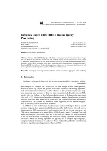
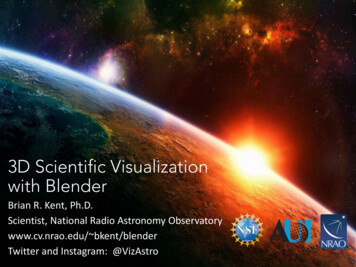
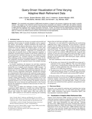
Fig. 2: This figure illustrates the sequential process of compositing the AMR grid hierarchies of two selected timesteps. The process begins by filling the composite template with allgrid cells, from both timesteps, of the finest level of refinement. In each subsequent pass, our procedure adds grid cells of the next level of lesser refinement to the template - conditionedon the basis that a more finely refined grid cell has not already been placed at that position. Finally, we add grid cells of the coarsest level of refinement to the template.resident in the template at this given location. This strategy continuesuntil the process conditionally adds grid cells of refinement level equalto l0 . Figure 2 illustrates this construction process.This refinement-level ordered compositing guarantees two fundamental properties in the final composite template: The template maintains the finest level of refinement from eachtimestep utilized in its construction – the template thus preservesthe high fidelity data created by the numerical simulation. The composite template provides a basis for resolving the differences in grid cell refinement that exist when a given point inspace is covered by different grid cell refinement levels at different points in time. Specifically, every grid cell from any AMRgrid hierarchy used to construct the composite template can bemapped to a grid cell of equivalent refinement, or a group ofnested grid cells of greater refinement, in the composite template.3.2.2 Grid SynchronizationThe composite template provides the common grid hierarchy necessary for performing query-driven analysis and multitemporal visualization of AMR data. The variable attributes (e.g. pressure, density,etc.) contained in each timestep’s grid hierarchy must now be synchronized with this template. The second fundamental property of thecomposite template formulates this synchronization process.Those grid cells (from all grid hierarchies used to generate the composite template) that map to regions of greater refinement in the composite template are synchronized through a regridding process. Thisregridding process iteratively divides the grid cell in question into anested group of grid cells of increased refinement. This refinementcontinues iteratively until grid cells are identical in refinement and hierarchical ordering to the group of nested grid cells in the compositetemplate. To complete the synchronization, we propagate the cell centered value of the original grid cell to the centers of the newly createdgrid cells. Figure 3 illustrates this process. With each timestep’s gridhierarchy synchronized, multitemporal query-driven visualization ofAMR data is now possible.3.3 Query-Driven Visualization of Temporal AMR DataThe goal of query-driven analysis is to provide scientists with interactive and resource-efficient methods for visually exploring large multidimensional data. To meet these needs, it is important to processuser’s queries, and render the results generated from these queries, asfast as possible. We meet these needs by employing a GPU-basedquery indexing structure, called the Bin-Hash index [10]. By utilizinga GPU-based query engine, we can implement the entire QDV process on the GPU and accelerate QDV performance as a whole withthe GPU’s parallel processing power. In our implementation, the CPUserves as a host to the GPU, only streaming the minimal data necessary to perform full-resolution queries (Section 3.3.2). All queries areevaluated (and rendered) on the GPU by executing kernels written inNVIDIA’s data-parallel programming language CUDA [22]. QDV inliterature typically evaluates scalar data. However, the Bin-Hash indexcan also evaluate vector data, as well as evaluate an arbitrary numberof timesteps or variables.The integration of the Bin-Hash index into QDV is similar to previous integrations that utilized a CPU-based index [26]. Both strategiesuse index building, index searching, record processing, and renderingprocedures. The difference between our work and previous work isthat we query and render adaptively refined spatiotemporal data. Thisdifference requires, in addition to the use of the composite templateand synchronized grid hierarchies (Section 3.2), mapping query results to direct the rendering of grid cells during the rendering stage.We discuss Bin-Hash index building, searching, and rendering next.3.3.1 Bin-Hash Index ConstructionThe strategy of the Bin-Hash method is based upon the observationthat query performance can be accelerated through the utilization ofmulti-resolution information. Supporting this approach requires twolevels of informational representation for the AMR data records: fullresolution (the 32-bit base data) and low-resolution information (8-bitencoded data).The Bin-hash index construction algorithm takes as input the fullresolution AMR data from a single timestep and generates both anencoded and spatially compacted version of this input. The index construction algorithm performs this operation in two stages. In the firststage, it utilizes a binning strategy to generate a binned (ı.e. encoded)version of the data. In the second stage it utilizes a combination ofdata partitioning with a technique referred to as spatial hashing [17]to compactly represent the full-resolution data contained in each binpreviously created by the first stage’s binning procedure.The first stage in the index construction process begins by examining and binning – independently – the data from each selectedtimestep’s hierarchy. For example, given a set of bin boundaries on avariable A, such as (b0 , b1 , . . . , bn ), each bin is defined to be the interval (b0 A b1 ), (b1 A b2 ), and so on. Bin-Hash binning alwaysutilizes 256 bins, where each bin contains approximately the samenumber of records. The encoded version of the dataset, referred to aslow-resoution data, is created by replacing each 32-bit full-resolutiondata value with its associated 8-bit bin number (0-255).The second stage in the process of index construction requires thepartitioning and spatial compaction of the original full-resolution data.Fig. 3: This figure depicts the sequential process of synchronizing the grid hierarchy ofa given timestep with a composite template. At each level of synchronization, grid cellsconditionally refine themselves by one additional level according to whether or not they aresynchronized with the composite template. In this example, synchronization is completefor the grid hierarchy in the second level of synchronization.

(a)(b)(c)Fig. 4: These images depict the three transfer functions we employ in our work. In (a)and (b) the colors correspond to levels of AMR grid refinement for the respective ArgonBubble and Hurricane datasets: green colors indicate grid cells of finest refinement, andgray colors indicate grid cells of coarsest refinement. In (c) the colors are used to conveysummary statistic information in multitemporal visualizations: blue colors indicate regionswhere few queries have selected a cell during QDV analysis, and yellow colors indicateregions where the most queries have selected the cell.To perform this, records are first partitioned according to their binnumbers. Next, these subsets of data are spatially compacted througha technique called perfect spatial hashing [17]. Perfect spatial hashing takes all the full-resolution data associated with the records of agiven bin, and stores it separately as two small tables: a hash table andan offset table. This operation is performed for all 256 bins. Oncethe second stage is completed, the total full-resolution dataset is nowrepresented as 256 pairs of hash and offset tables. The total storageoverhead for the indices is approximately 1.5 - 2.0 times the size ofthe original AMR data. This partitioning and spatial hashing of thedata is essential to the search process as the next section details.3.3.2 Bin-Hash Index SearchingBefore

We present a new method for performing query-driven visualization and analysis on AMR data, with specific emphasis on time-varying AMR data. Our work introduces a new method that directly addresses the dynamic spatial and temporal properties . data. Park et al. [23] present a hierarchical multi-resolution splatting technique for AMR data .