Transcription
Adv Comput Math (2011) 34:67–81DOI 10.1007/s10444-009-9142-7The missing Wendland functionsRobert SchabackReceived: 13 November 2008 / Accepted: 12 September 2009 /Published online: 24 September 2009 The Author(s) 2009. This article is published with open access at Springerlink.comAbstract The Wendland radial basis functions (Wendland, Adv Comput Math4:389–396, 1995) are piecewise polynomial compactly supported reproducingkernels in Hilbert spaces which are norm–equivalent to Sobolev spaces. Butthey only cover the Sobolev spacesH d/2 k 1/2 (Rd ), k N(1)and leave out the integer order spaces in even dimensions. We derive themissing Wendland functions working for half-integer k and even dimensions,reproducing integer-order Sobolev spaces in even dimensions, but they turnout to have two additional non-polynomial terms: a logarithm and a squareroot. To give these functions a solid mathematical foundation, a generalizedversion of the “dimension walk” is applied. While the classical dimension walkproceeds in steps of two space dimensions taking single derivatives, the newone proceeds in steps of single dimensions and uses “halved” derivatives offractional calculus.Keywords Sobolev spaces · Compactly supported radial basis functions ·Kernels · Hypergeometric functions · Positive definite functions ·Fractional calculusMathematics Subject Classifications (2000) 33C90 · 41A05 · 41A15 · 41A30 ·41A63 · 65D07 · 65D10Communicated by Joe Ward.R. Schaback (B)Institut für Numerische und Angewandte Mathematik, Universität Göttingen,Lotzestrasse 16–18, 37083 Göttingen, Germanye-mail: schaback@math.uni-goettingen.de
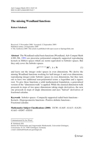
68R. Schaback1 IntroductionIn a wide range of applications from Machine Learning to Meshless Methods[11], positive definite kernels have proven to be very useful tools. They arisenaturally as reproducing kernels of Hilbert spaces of continuous functions,and they often come in translation- and rotation-invariant form as radial basisfunctionsK(x, y) φ( x y 2 ) for all x, y Rdon Rd with a smooth univariate function φ : [0, ) R. Typical examplesare furnished by the Gaussian φ(r) : exp( r2 ) or the Sobolev/Matérn functions φ(r) Kν (r)rν . The latter have special importance in geostatistics [8], andare the reproducing kernels of Sobolev spaces H m (Rd ) for ν m d/2 0.They involve the Kν Bessel functions of third kind and decay exponentiallytowards infinity.Unfortunately, these kernels are not compactly supported, but by arguments using convolutions of compactly supported functions, it is quite clearthat there must be compactly supported positive definite radial basis functionsof arbitrary prescribed smoothness. The quest for explicit formulas for suchfunctions started with “Euclid’s hat” in 1993 [4, 9] and continued with piecewise polynomial radial basis functions of Wu [16] and Wendland [14] in 1995.While Euclid’s hat is not differentiable and Wu’s functions have zeros in theirFourier transform, Wendland’s functions φd,k have no such drawbacks. Theyare polynomials on [0, 1] and yield positive definite C2k radial basis functionson Rd . Given these properties, their polynomial degree d/2 3k 1 isminimal, and they are reproducing kernels of Hilbert spaces isomorphic toSobolev space H d/2 k 1/2 (Rd ).But since this means that integer-order Sobolev spaces in even dimensionsare not covered, this paper produces the “missing” functions by allowinghalf-integer values of k. They still are compactly supported, but they arepolynomials with additional logarithmic and square-root terms. For example,the function 2r(2) (2r2 1) 1 r2φ2,1/2 (r) 3r2 log 3 π1 1 r2on [0, 1] and extended by zero to [0, ) yields a positive definite radialbasis function on R2 and it will turn out to be the reproducing kernel in anisomorphic copy of to H 2 (R2 ). See Fig. 1 for a plot of this function.The paper will first review the standard construction process for Wendland’sfunctions by the “dimension walk”. It usually steps through space dimensionsin steps of two while taking successive derivatives. To reach the missingintermediate space dimensions, the dimension walk has to proceed in stepsof single dimensions. But then it has to use “half-derivatives” from what iscalled “fractional calculus” [7]. This generates the functions we need, and we
Wendland functionsFig. 1 The missing Wendlandfunction φ2,1/2690.250.20.150.10.0500.20.40.60.81xprovide a MAPLE program for explicit calculation. Finally, we add proofs forthe required properties of the new functions and close with an outlook thatconnects everything to hypergeometric functions.2 Radial transformsTo start with, we repeat part of the machinery of fractional calculus from [12]and [10]. Proof details can be found there. It is well-known that a radial basisfunction (x) : φ( x 2 ), x Rdhas a radial d-variate Fourier transform (d 2)/2ˆ (ω) ω 2 φ(r)rd/2 J(d 2)/2 (r ω 2 )dr(3)0if the integral exists. It allows the Fourier transform of a radial function to bewritten as a univariate Hankel transform.We now introduce t r2 /2 as a new variable, writing a radial basis functionφ asφ( · 2 ) f ( · 22 /2).(4)At first sight, this “ f -form” seems somewhat strange. Indeed, the f -formof the familiar Wendland function φ3,1 (r) (1 r)4 (4r 1) will be the non polynomial function f3,1 (t) (1 2t)4 (4 2t 1). But the following mathematical analysis of radial functions in f -form turns out to be much simplerthan in “normal” form, and this fact should be familiar from Schoenberg’sconnection of positive definite radial basis functions to completely monotonefunctions [13].
70R. SchabackNow (3) for ν (d 2)/2, when written in f -form on both sides, turns into f (t)tν Hν (ts)dt(5)(Fν f )(s) : 0with the function z ν2Jν (z) : Hν (z2 /4) k 0( z2 /4)kk! (k ν 1)(6)for z C and ν C with ν 0. Note that (5) is a generalization of the Fouriertransform on radial functions, allowing Fourier transforms for spaces of fractaldimension, because ν (d 2)/2 need not be a half-integer. The functions z νJν (z) Hν (z2 /4)2are called oscillatory radial basis functions by Fornberg et al. [3]. The abovederivation shows that they are of central importance, because they supply thegeneralized Fourier transforms of general radial functions. We shall use themfrequently in what follows.Using derivative formulae for the Hν functions obtainable from those of theJν functions, one gets dFν ( f )(s) Fν 1 ( f )(s) and (Fν 1 ( f ))(s) (Fν ( f ))(s).ds(7)Going back to ν (d 2)/2, these are the basic features of the dimensionwalk, but we shall need them later in steps of dimension one:Theorem 1 If the mentioned Fourier transforms and derivatives exist,––the (d 2)-variate Fourier transform of a radial function after the f -formsubstitution (4) is the negative univariate derivative of the d-variate Fouriertransform in f -form, andthe d-variate Fourier transform of a radial function in f -form is the (d 2)variate Fourier transform of the negative derivative of f .Note that all continuous and compactly supported f will have smoothgeneralized Fourier transforms Fν ( f ) in all dimensions, making the left-handpart of (7) valid for all dimensions. However, the application of the right-handpart of (7) is restricted by the smoothness of f .The dimension walk, expressed via derivatives, is extremely useful whenprogramming with radial basis functions. It turns out that all the relevantclasses of radial basis functions, when written in f form, are invariant underdifferentiation and integration, while the Fν operators map the class to anotherone which is also closed under differentiation and integration. Implementingthe general class in f form automatically yields an implementation of allderivatives.
Wendland functions71But we shall need fractional derivatives to generalize all of this. To this end,[12] introduces a scale of integral operators (s t)α 1(8)dsIα ( f )(t) : f (s) (α)tfor all α 0, t 0, defined on continuous functions on [0, ) with compactsupport or exponential decay at infinity. As the authors of [12] found outlater, these are closely connected to the Weyl derivative operators of fractionalcalculus and were introduced also in [6] for use in the dimension walk. Thesimplest special case is I1 ( f )(t) : f (s)dstwith the inverseI 1 ( f )(r) : f (r)we already had above, doing the dimension walk. These operators satisfyIα Iβ Iα βfor all α, β 0. Thus the “semi-integration” operator f (s)dsI1/2 ( f )(t) π(s t)tsatisfies I1/2 I1/2 I1 . These definitions can be extended to letIα Iβ Iα βhold for all α, β R and on suitable domains, but we refer to [10, 12] fordetails. Note that all of these operators are intended to work on f -forms ofradial functions, not on their normal form. They are closely connected but notidentical to the standard operators of fractional calculus.With these operators at hand, [10, 12] generalize the dimension walk to(Fμ Fν )( f ) Iν μ ( f )Fμ Iν μ FνFν Fμ Iν μ(9)as far as the operators are applicable, in particular for ν μ and on compactlysupported smooth functions, and this is what we need for generating themissing Wendland functions.3 Application to Wendland functionsDue to a result of Askey [1] the radial truncated power functionsμAμ (·) : (1 · 2 )
72R. Schabackare positive definite on Rd for integer μ d/2 1, because they have astrictly positive radial Fourier transform in these cases. Formally, we allow μto be positive and real from now on and turn to positive definiteness later.The f -form of Askey functions is μaμ (s) : (1 2s) .Since the Iα operators preserve compact supports and are applicable to aμ forall α, μ 0, we can defineaμ,α : Iα (aμ ) with aμ,0 aμ .Going back to “normal” form, the functionsψμ,α (r) : (Iα (aμ ))(r2 /2))(10)are well-defined and supported in [0, 1] for all α, μ 0 and can be called general Wendland functions. At this point, we do not know for which parametersthey are positive definite in which space dimension. They can be represented as ψμ,α (x) 0 1 x(1 μ (s x2 /2)α 1 2s) ds (α)t(1 t)μ(t2 x2 )α 1dt (α)2α 1(11)for x [0, 1]. This coincides with the formula (9.2.20) in [10] (see also Gneiting[5]) and it is normally used only for integer α, μ to get the polynomialrepresentations of the Wendland functions directly. The connection to the φd,knotation in Wendland’s monograph [15] to the above formula is viaφd,k ψ d/2 k 1,k ,(12)because there are good reasons to pick the smallest known μ which guaranteesψμ,k to be positive definite in d dimensions for a given d, and this minimal μis d/2 k 1 for integer k. The case of half–integer α or μ of the formula(11) was not treated so far, though it clearly generates functions with supportin [0, 1].4 Construction algorithmIf μ and α are integers, the resulting function in (11) is a single polynomial ofdegree μ 2α in the variable x · 2 on its support, and the integral can be
Wendland functions73directly calculated. However, one can try to calculate the integral in general,and this is partially done by the MAPLE snippetwend: proc(mu,alpha,x)local wend;wend: r*(1-r) mu*(r*r-x*x) (alpha-1)/(GAMMA(alpha)*2 (alpha-1));wend: int(wend,r x.1);return factor(simplify(wend));end proc:which runs for all reasonable and fixed choices of μ and α where one halfinteger is allowed, while it fails if both μ and α are genuine half-integers. Sinceψd/2 α 1/2,α φd,α will be proven in Corollary 1 below to be reproducing inspaces norm-equivalent to H d/2 α 1/2 (Rd ) for half-integer α and even d, theabove snippet generates the missing Wendland functions for half-integer α andinteger μ. The first interesting case is μ d 2, α 1/2 leading to (2) plottedin Fig. 1. It is a reproducing kernel in an isomorphic copy of H 2 (R2 ). Using theabbreviations xL(x) : log 1 1 x2(13) 2S(x) : 1 xthe next cases areψ2,3/2 (x) ψ2,5/2 (x) ψ4,1/2 (x) ψ4,3/2 (x) 2 15x4 L(x) (8x4 9x2 2)S(x) ,60 π 2 105x6 L(x) (48x6 87x4 38x2 8)S(x) .2520 π 2 (45x4 60x2 )L(x) (16x4 83x2 6)S(x) ,30 π 2 (105x6 210x4 )L(x)420 π (32x6 247x4 40x2 4)S(x) , 2ψ4,5/2 (x) (945x8 2520x6 )L(x)30240 π (256x8 263x6 690x4 136x2 16)S(x) , 2 ψ6,1/2 (x) (525x6 2100x4 840x2 )L(x)280 π (128x6 1779x4 1518x2 40)S(x) .
74R. SchabackThe general case will be proven below to be of the formψ2m,(2 1)/2 (x) x2 pm, (x2 )L(x) qm, (x2 )S(x)(14)with polynomials pm, of degree m 1 and qm, of degree m 1 .These functions do not seem to be directly available via the technique ofBuhmann [2].5 Theoretical analysisWe now provide rigid proofs of the statements made above. Recall that thestandard Askey functions satisfy Fν (aμ ) 0 iff μ ν 2 where μ is aninteger and ν (d 2)/2 may be a half-integer. Furthermore, we know thatFν ( f ) 0 and d 2ν 2 N imply that f ( . 22 /2) is positive definite onRd R2ν 2 .Theorem 2 For all α N/2 and all μ N withμ d/2 α 1,(15)the generalized Wendland function ψμ,α is positive definite on Rd .Proof We use the identity Fν α Fν Iα from (9) for aμ and getFν α aμ Fν (Iα (aμ ))(16)which is valid for all α, μ 0 and all ν 1/2. But we restrict ourselves tothe caseν α Z/2, ν α 1/2,and apply Askey’s result for d 2ν 2α 2 to get that the left-hand side isstrictly positive wheneverμ ν α 2.Looking at the right-hand side of (16) and introducing a new dimension with(d 2)/2 ν, we see that the function Iα (Aμ ) is positive definite on Rd if (15)holds. Theorem 3 For α N/2, the d-variate Fourier transform Fd (ψμ,α ) of ψμ,α withμ d/2 α 1 3(17)satisfiesFd (ψμ,α )(r) (d 2α 1)rfor r .(18)
Wendland functions75Proof Using (16) and the transition to the f -form, we getFd ψμ,α (r) F d 2 aμ,α (r2 /2)2F d 2 α aμ,0 (r2 /2)2Fd 2α aμ (r2 /2)Fd 2α Aμ (r)(19)to see that the d-variate Fourier transform of ψμ,α in normal form is identicalto the (d 2α)-variate Fourier transform of the Askey function Aμ in normalform.Since (17) allows two possible connections between μ and d, we fix d andα first, define d : d 2α and look at the two possibilities d 2μ 1 andd 2μ 2 which share d /2 d/2 α μ 1. From section 10.5 of [15]we cite(F2μ 1 Aμ )(r) (F2μ 2 Aμ )(r) (r 2μ )(r 2μ 1 )for integer μ 3. Then (19) yields the assertion.(20) Note that the above argument excludes μ 2, α 1/2 and d 1, thus notproving that ψ2,1/2 is reproducing in a space equivalent to H 3/2 (R1 ). But itgeneralizes (1) for half-integers α and even-dimensional spaces, since μ 3holds in such cases:Corollary 1 For integers m 1 and n 0, the generalized Wendland functionψm n 1,n 1/2 taken for even dimensions d 2m is reproducing in a Hilbert spacewhich is isomorphic to Sobolev space H m n 1 (R2m ) H d/2 α 1/2 (Rd ) whereα n 1/2.6 Inductive constructionThis chapter proves the representation (14) for the missing Wendland functions ψ2m,(2 1)/2 for all and m. We start with 1 and general m.Theorem 4 The general Wendland functions a2m,1/2 (t) have the form 1/2(1 2s)2mdsa2m,1/2 (t) : π(s t)t Pm,0 (t)L( 2t) Qm,0 (t)S( 2t)with polynomials Pm,0 , Qm,0 of degree m andPm,0 (1/2) Qm,0 (1/2)Pm,0 (0) 0for all m 1.(21)
76R. SchabackProof We can also consider 12r(1 r)2mdra2m,1/2 (x /2) π xr 2 x2 Pm,0 (x2 /2)L(x) Qm,0 (x2 /2)S(x) and transform this by z : r2 x2 into 1 x22a2m,1/2 (x2 /2) (1 x2 z2 )2m dz.π 02Applying the binomial formula leads to terms gk (x) : 1 x2(x2 z2 )k dz0for all k Z/2 with 0 k m combining into 2m 2 2m2g j/2 (x).a2m,1/2 (x /2) ( 1) jjπ j 0We get gk 1 (x) 1 x2(x2 z2 )(x2 z2 )k dz 1 x2 x2 gk (x) z2 (x2 z2 )k dz 0 1 x21 x212 x gk (x) (x2 z2 )k 1 dz2(k 1)2(k 1)0 11 x22 gk 1 (x) x gk (x) 2(k 1) 2(k 1)0such that 1 x2 x gk (x) 2(k 1)2k 2 2S(x)gk 1 (x) x gk (x) 2k 32k 31gk 1 (x) 1 2(k 1) 2is a useful recursion that boils everything down to S(x)g0 (x) 1 x2 21 11 xg1/2 (x) x2 L(x) S(x) x2 L(x) .222This gives polynomials p j, q j, r j of degree at most j withg j(x) S(x) p j(x2 )g j 1/2 (x) L(x)q j(x2 ) S(x)r j 1 (x2 )(22)
Wendland functions77such that m π2m2gi (x) a2m,1/2 (x /2) 2i2i 0 m 2mgi 1/2 (x) 2i 1i 1 m m 2m2m2pi (x ) ri 1 (x2 ) S(x)2i2i 1i 0i 1 m 2m2 L(x)qi (x )2i 1i 1is of the required form.We have to check the additional conditions (21). Since q j has no constantterm, we get Pm,0 (0) 0. To prove the conditions at 1/2, we remark thatevaluation of an f form at 1/2 means evaluation of the standard form at 1.We rewrite the representation (22) in terms of z 1 x2 as a2m,1/2 ((1 z2 )/2) Pm,0 ((1 z2 )/2)L( 1 z2 ) Qm,0 ((1 z2 )/2)S( 1 z2 )and now evaluation at x 1 means evaluation at z 0. We expand the termsat z 0 to get L( 1 z2 ) z O (z3 )S( 1 z2 ) zto see thata2m,1/2 (1/2) Pm,0 (1/2) Qm,0 (1/2)which vanishes due to the support of the f form ending at 1/2. Theorem 5 The representationa2m,(2 1)/2 (s) Pm, (s)L( 2s) Qm, (s)S( 2s)(23)with polynomials Pm, , Qm, of degree m andPm, (1/2) Qm, (1/2)Pm,0 (0) 0holds for all m 1 and all 0.Proof We know that (23) holds for 0 and all m 1, and thus we proceed byinduction on . By the standard dimension walk rules (9) we have to constructPm, , Qm, from Pm, 1 , Qm, 1 to satisfy a2m,2 1 (s) a2m,(2 1)/2 (s).(24)
78R. SchabackThe induction recipe will be to define Pm, byPm, (s) Pm,Pm, (0) 0 1 (s)(25)and to define Qm, viaQm, (s) (1 2s) Qm, (s) Pm, (s) Qm,2s 1 (s)(1 2s).It can easily be shown that the above equation is uniquely solvable for Qm, ofdegree m , and it impliesQm, (1/2) Pm, (1/2).Now we have to evaluate both sides of (24) in order to finish the induction. Weneed the derivatives1L (x) x 1 x2 xS (x) 1 x2 1L( 2s) 2s 1 2s 1S( 2s) 1 2sand geta2m,(2 1)/2 (s) Pm, (s) L( 2s) Pm, (s)L( 2s) Qm, (s) S( 2s) Qm, (s)S( 2s) 1 Pm, (s) L( 2s) Pm, (s) 2s 1 2s 1 Qm, (s) S( 2s) Qm, (s) .1 2sFocusing on the log terms above and in a2m,(2 1)/2 (s), we see that they arecorrect due to our choice of Pm, . Now we are left to prove that Qm, 1 (s)S( 2s) Qm, 1 (s) 1 2scoincides withPm, (s) 11 Qm, (s) 1 2s Qm, (s) . 2s 1 2s1 2sBut the latter is identical toPm, (s) 2s(1 2s)Qm, (s) 2sQm, (s). 2s 1 2s
Wendland functions79 Introducing z : 1 2s we have to prove 1 z211 z2 Qm, 1z Pm,2z(1 z2 )2 2 1 z1 z222 Qm,z (1 z ) Qm,(1 z2 ).22But since our construction yieldsPm, (1/2) Qm, (1/2)Pm, (0) 0, the critical denominator cancels, and our definition of Qm, does the job.Note that Theorems 4 and 5 imply the representation (14). The special formof the pm, part is due to the fact that (25) does not change the number ofmonomial terms, which is fixed at startup in Theorem 4, but only blows thedegree up by one.7 Open problemsReaders will have noticed that we did not deal with the two remaining casesof generalized Wendland functions ψμ,k : those with integer k and half-integerμ and those with both indices being half-integer. We did not focus on thesebecause they are less promising. This is based on some hypotheses, confirmedfor special cases, which we now formulate.First, there is quite some evidence that ν 3/2tFν (aμ,0 )(t) for t (26)holds in full generality, in particular independent of μ, and is positive for all3μ ν ,2(27)not only in the special cases related to (20). Note here that the standard case isrecovered by ν 3/2 d/2 1/2 d/2 1 if ν (d 2)/2,but one could allow more general ν. The above assertions should follow froma very thorough inspection of chapters 6 and 10 of [15], and they generalizeTheorems 2 and 3. Since large μ do not pay off, Wendland’s notation (12)based on the smallest μ yielding positive definiteness for dimension d makes alot of sense.If the above is assumed, the minimal μ for ψμ,α to be positive definite ingeneralized dimension d isμ α d/2 1/2 .
80R. SchabackThen (26) can be applied for ν α (d 2)/2, proving that the generalizedWendland function ψ α d/2 1/2 ,α is reproducing in Hilbert spaces isomorphicto H m (Rd ) for m α d/2 1/2. This should be expected for all real d andα, leading to compactly supported reproducing kernels also in fractional-orderSobolev spaces.To generate the integer-order Hilbert spaces in all dimensions, it thereforesuffices to use the classical Wendland functions and those we described here.The μ parameter is not of central importance. However, fractional Sobolevspaces will require fractional α, but our integral operators (8) will allow togenerate these either directly via (10) and (11), if the integral can be calculated,or from a polynomial Wendland function viaIα aμ Iα α I α aμ Iα α aμ, α if the operator Iα α can be explicitly evaluated on monomials.The case of ψμ,α with half-integer μ (N/2) \ N and integer α can easily behandled with the methods of Section 4 and the MAPLE program presentedthere. It generates polynomials times 1 x. But under the above assertions,genuinely half-integer μ do not seem to be minimally chosen. Things would bedifferent if there was half-integer leeway in the condition (27), but F1/2 a7/4,0 isnot positive, thanks to MAPLE.Finally we remark that there are good chances to put all of this into auniform theory based on hypergeometric functions. But we leave these thingsopen.AcknowledgementSpecial thanks go to a referee for careful reading and useful suggestions.Open Access This article is distributed under the terms of the Creative Commons AttributionNoncommercial License which permits any noncommercial use, distribution, and reproduction inany medium, provided the original author(s) and source are credited.References1. Askey, R.: Radial characteristic functions. Technical Report 1262, Univ. of Wisconsin, 1973.MRC Technical Sum. Report.2. Buhmann, M.D.: Radial functions on compact support. Proc. Edinb. Math. Soc. 41, 33–46(1998)3. Fornberg, B., Larsson, E., Wright, G.: A new class of oscillatory radial basis functions. Comput.Math. Appl. 51(8):1209–1222, 2006.4. Gneiting, T.: Radial positive definite functions generated by Euclid’s hat. J. Multivar. Anal.69(1), 88–119 (1999)5. Gneiting, T.: Compactly supported correlation functions. J. Multivar. Anal. 83(2), 493–508(2002)6. Matheron, G.: Les Variables régionaliseés Et Leur Estimation. Masson, Paris (1965)7. Oldham, K.B., Spanier, J.: The Fractional Calculus; Theory and Applications of Differentiation and Integration to Arbitrary Order. Academic, London (1974)8. Pardo-Iguzquiza, E., Chica-Olmoa, M.: Geostatistics with the matern semivariogram model:a library of computer programs for inference, kriging and simulations. Comput. Geosci. 34,1073–1079 (2008)
Wendland functions819. Schaback, R.: Creating surfaces from scattered data using radial basis functions. In: Lyche, T.,Daehlen, M., Schumaker, L.L. (eds.) Mathematical Methods for Curves and Surfaces, pp. 477–496. Vanderbilt University Press, Nashville (1995)10. Schaback, R.: Reconstruction of multivariate functions from scattered data. chaback/research/group.html (1997)11. Schaback, R., Wendland, H.: Kernel techniques: from machine learning to meshless methods.Acta Numer. 15, 543–639 (2006)12. Schaback, R, Wu, Z.: Operators on radial basis functions. J. Compt. Appl. Math. 73, 257–270(1996)13. Schoenberg, I.J.: Metric spaces and completely monotone functions. Annal. Math. 39, 811–841(1938)14. Wendland, H.: Piecewise polynomial, positive definite and compactly supported radial functions of minimal degree. Adv. Comput. Math. 4, 389–396 (1995)15. Wendland, H.: Scattered Data Approximation. Cambridge Monographs on Applied andComputational Mathematics. Cambridge University Press, Cambridge (2005)16. Wu, Z.: Compactly supported positive definite radial functions. Adv. Comput. Math. 4, 283–292 (1995)
Wendland functions 69 Fig. 1 The missing Wendland function φ2,1/2 0 0.05 0.1 0.15 0.2 0.25 0.2 0.4 0.6 0.8 1 x provide a MAPLE program for explicit calculation. Finally, we add proofs for the required properties of the new functions and close with an outlook that connects everything to hypergeometric functions. 2 Radial transforms