Transcription
ESTEEM, Vol. 4, No. 2, 2008, 3-14Using Kaplan Meier and CoxRegression in Survival Analysis:An ExampleTeoh Sian HoonABSTRACTThe Kaplan Meier procedure is used to analyze data based on the survivaltime. This article provides an example on how to use Kaplan Meier and Coxregression with three objectives. The objectives are finding the percentage ofsurvival at any time of interest, comparing the survival time of two studiedgroups and examining the effect of continuous covariates with the relationshipbetween an event and possible explanatory variables. The example is discussedbased on the breast cancer survival dataset from Statistical Package for theSocial Sciences (SPSS).Keywords: Survival time, the Kaplan Meier procedure, Cox regressionIntroductionThis article provides an example on how to use the Kaplan Meierprocedure and Cox regression to analyze data with censored data onsurvival time as well as to find the relationship between an event andpossible explanatory variables. The procedures in the Kaplan Meier andthe Cox regression were reviewed in the following literature review.Using the Cox regression model to find the effects of covariates requiresthe use of a statistical software package because straightforward singleequation for the estimation is not available (Daniel, 2005). In this paper,the software package SPSS (Statistical Package for the Social Sciences)was used. After the data are included in the analysis using SPSS, thedata are analyzed based on the procedures.Literature ReviewSurvival analysis is used to analyze data corresponding to survival time.Survival time is the time taken when an end event occurs in the data set.3
Teoh Sian HoonThus, it is the time to events, and is also known as failure-time data orthe end point. Time to events include survival time in medical events andnon-medical events. An example of survival time in a medical event isthe survival time until death or until being discharged from hospital.Another good example is the time for a tooth experiences carries asdiscussed in a longitudinal oral health study (Komarek, Lesaffre,Harkanen, Declerck & Virtanen, 2005; Lesaffre, 2005). On the otherhand, an example of survival time in non-medical event is the time fromgraduation until one gets a job. A famous example of the application ofsurvival analysis for non-medical event is finding the determinants of thesurvival of a network in franchising, where time is an important variablefor the development of franchising (Perrigot, Cliquet and Mesbah, 2004).All the cases in the above examples have data consist of censoredobservations in which the end event has not happened in every observationor when information on a case is only known for a limited duration. Thecensoring time is the main information to find cumulative survivalprobability in the survival analysis. In other words, the great advantageof using survival analysis is to analyze censored cases in analysis.The Kaplan-Meier procedure (Kaplan & Meier, 1958) is used tocalculate the survival rate from the survival function. It involves estimatingthe probability of surviving for a specified length of time. The advantageof using Kaplan-Meier curves is that they are non-parametric, where noassumptions are made on the distribution of survival times (Kaplan &Meier, 1958; Daniel, 2005). The survival function is the number ofindividuals with survival time, which is at least t time periods divided bythe number of individuals in the study. The Kaplan-Meier estimate of thesurvival function is a product-limit estimate as indicated in Equation 1,s(t) U Vj i(i)"Jwhere n. number of individuals alive just before time t(), and d. number of deaths at tQ for t(k) t t(k ]), and k 1,2, ., r.The two useful regression models, namely linear regression modelsand logistic regression model are used for continuous outcome measuresand binary outcome measures. Cox regression or proportional hazardregression is an additional type of regression models. It is used when thedependent observations consist of a mixture of either time-until-eventdata or censored time observations (Daniel, 2005). The function involvedis hazard function, which describes the conditional probability of an4
Using Kaplan Meier and Cox Regressionindividual who has survived to time t and will die in the next small periodof time. The Cox proportional hazard model assumes that the hazardsfor two groups are proportional (Collet, 2003). The regression model isdescribed in Equation 2.h(t,x i ) e f ( x ' ) h 0 (t)(2)f(x )where e v ,J indicates how different covariates affect survival (i.e.,compares the hazard to the baseline) and ho(t) is an arbitrary baselinehazard function that is assumed to be the same for all groups.By rearranging the Equation 2, we can get the exponentiatedcoefficient, which represents the hazard ratio for the basis in proportionalhazard regression as indicated in Equation 3.M i) e f(x i )ho(t).(3)ObjectivesThere are three main objectives in the following discussion. They are(1) to find the percentage of survival at any time of interest, (2) to comparethe survival time of two studied groups, and (3) to examine the effects ofcontinuous covariates. The Kaplan Meier procedure was used for thefirst and second objectives. Cox regression was used for the thirdobjective.MethodologySPSS was used in this analysis. Kaplan Meier and Cox regression arethe two main analyses in this paper. The Kaplan Meier procedure isused to analyze on censored and uncensored data for the survival time.It is also used to compare two treatment groups on their survival times.The Kaplan Meier technique is the univariate version of survival analysis.To present more details in the survival analysis, further analysis usingCox regression as multivariate analysis is presented. Cox regressionallows the researcher to include predictor variables (covariates) into themodels. Cox regression will handle the censored cases correctly. It willprovide estimated coefficients for each of the covariates that allow us toassess the impact of multiple covariates in the same model. We can alsouse Cox regression to examine the effect of continuous covariates. The5
Teoh Sian Hoonsteps required in SPSS to perform the above objectives are listed asfollows.Variables UsedThe event of interest in a medical research using survival analysis isdeath due to a disease. There are two groups of status, which arecensored data and uncensored data. The occurrence of censoredobservations may due to a few reasons. Firstly, the observations are stillalive at the end of study for which the critical event has not yet occurred.Secondly, the observations' follow-up information are lost. This can becaused by the person's reluctance to turn up for the following study daysafter committing to the study. Thirdly, the event occurs but the cause isunrelated to the disease.The status of data is recorded to identify whether the observation is acensored data or an uncensored data. For censored data, the status isdenoted as '0'. For uncensored data, the case from an event of dying fromthe disease is denoted as ' 1'. Normally a factor is used to indicate whetherthe observation is in the treatment group or control group. If there are onlyone treatment group and one control group, the factor is set as '0' forcontrol group and' 1' for the treatment group. But, if there are two treatmentgroups and one control group, '0' is set for the control group,' 1' is set forthe first treatment, and '2' is set for the second treatment.The event of interest in this study is death due to breast cancer. Afew variables were used in this discussion. Firstly, status of a variablewas used to indicate the status of censored data or uncensored data.Status of '0' denotes censored data and status ' 1 ' denotes uncensoreddata. Secondly, variable time was used to indicate time of occurrencefor censored and uncensored observations. Thirdly, variable Lymph Nodeswas included as a factor to compare the survival times of two groups. Inthis example, factor Lymph Nodes has two categories. They are statusof 'No' for not having Lymph Nodes and status of 'Yes' for havingLymph Nodes. In the data set, '0' was recorded to define the status of'No' and ' 1 ' was recorded to define the status of 'Yes' for the factorLymph Nodes. Fourthly, variables age, Histologic Grade and LymphNodes were used as covariates in a further analysis, namely Coxregression.6
Using Kaplan Meier and Cox RegressionSteps for the First and Second Objectives: Using theKaplan Meier ProcedureKaplan Meier is used to analyze survival time data. The following stepswill give descriptive statistics for the survival time and a survival plot forthe survival function. Step 1 to step 4 are checked on to perform the firstobjective. Additional two steps, namely step 5 and step 6, are required toperform the second objective.Step 1:Step 2:Step 3:Step 4:Step 5:Step 6:From Menu bar, click on 'Analyze', point to 'Survival', followedby 'Kaplan Meier'.Select and move variable 'time' to the 'Time' box and variable'status' to the 'Status' box.Click 'Define Event' under 'Status' box, then, include ' 1' as anevent as defined and click 'Continue'.Click 'Option' button and mark on 'Mean and median survival'under 'Statistics' dialogue box; mark on 'Survival' under 'Plots'dialogue box.Select and move variable 'Lymph Node' to the 'Factor' option.Click 'Compare Factor.' button and click on 'Log rank'. Thenclick 'Continue' button.Steps for the Third Objective: Using Cox RegressionWe can determine whether the two groups differ with a few predictorvariables, namely Lymph Node, Histologic Grade and age by performingCox regression. The independent variables (covariates) can be continuousor categorical; for categorical variables, reference groups should beindicated. By default the last group is referred as the reference group.In this example, Histologic Grade and Lymph Nodes are categoricalvariables, the reference category for Histologic Grade is "3", and thereference category for Lymph Nodes is "1". The following steps willgive the estimated variables in Cox regression.Step 1:Step 2:Step 3:From Menu bar, click on 'Analyze', point t o ' Survival', followedby 'Cox Regression'.Select and move variable 'time' to the 'Time' box and variable'status' to the 'Status' box.Click 'Define Event' under 'Status' box, then, include ' 1' as anevent as defined and click 'Continue'.7
Teoh Sian HoonStep 4:Step5:Step 6:Select and move variable 'Lymph Node', 'Histologic Grade'and 'age' to the 'Covariates' box.Click 'Categorical.' button and include variables 'LymphNode' and 'Histologic Grade' into 'Categorical Covariates' box.Then, click 'Continue'.Click 'Options.' button and click on 'CI for exp(B)' checkboxin 'Cox Regression: Options' dialogue box.ResultsThe following results are presented according to the three objectives.Using the Kaplan Meier ProcedureTable 1, Table 2, and Figure 1 are presented as below for the analysisbased on the first objective. Table 1 shows the number of events, namelythe number of cases is 72, with the percentage of censored cases being94%. Table 2 shows the mean of survival time is 122.692 months, withthe standard error of 1.307 months. Figure 1 shows the survival plots. Itis shown in the diagram that at 70 months, 90% of the observations werestill alive. From Figure 1, more information on the percentage of thesurvival for different months can be accessed by referring to the specificmonth and looking for the associate survival rate.Table 1: Case Processing SummaryCensoredTotal NN of eventsNPercent1,207721,13594.0%Table 2: Means for Survival TimeMeana95% Confidence intervalEstimateStd. errorLower boundUpper bound122.6921.307120.131125.253* Estimation is limited to the largest survival time if it is censored.8
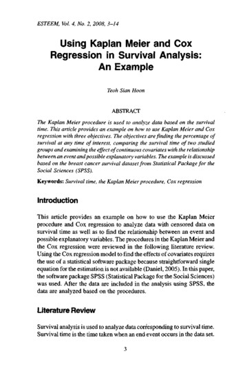
Using Kaplan Meier and Cox Regression1.0-« Survival Function - - 0120.00140.00Time (months)Figure 1: Survival FunctionTable 3, Table 4, Table 5 and Figure 2 are presented as below for theanalysis on the second objective. Table 3 shows the number of cases forthe two categories in Lymph Nodes, with cases of 'No' at 929 observationsand cases of 'Yes' at 278 observations. Thus, there are 929 observationswhich do not have Lymph Nodes and 278 observations which have LymphNodes. Table 4 shows the mean survival times for the two groups, withthe mean for cases of 'No' (without Lymph Nodes) as 124.920 monthsand the mean for cases of 'Yes' (with Lymph Nodes) as 111.331 months.Table 5 shows the results of log-rank test with thep-value of .000, whichindicates that there is a significant difference between the two groupson having a shorter time to event. The survival plot (Figure 2) shows thegroup without the Lymph Nodes has a longer survival time to eventcompared to the group with Lymph Nodes. This scenario is shown inFigure 2, whereby 92% of patients without Lymph Nodes were still aliveat 60 months as compared to 82% of patients with Lymph Nodes. FromFigure 2, more information on the survival rate for different months forthe two groups can be retrieved by referring to the specific month andlooking for the associated survival rates.9
Teoh Sian HoonTable 3: Case Processing Summaryyes or no(with LymphNodes)NoYesOverallCensoredTotal N9292781,207TV of e 4: Means for Survival TimeMeana(with LymphNodes)95% Confidence intervalEstimateStd. errorLower boundUpper 307122.177105.436120.131127.664117.226125.253Table 5: Overall ComparisonstLog Rank (Mantel-Cox)dfSig.1.00015.988Note: Test of equality of survival distributions for thedifferent levels of Lymph Nodes.Survival Functions1.00.92 -.rj ?c ?* » iWithout Lymph Node *»**—,.0.8-With Lymph Node— - m i l f H .-i--- iii. M .00120.001«0.00Time (months)Figure 2: Survival Plot for Comparison of the Two Groups10
Using Kaplan Meier and Cox RegressionResults from the Cox regression are presented in Table 6, Table 7,Table 8, and Table 9. Table 6 shows that only 76.2% of the observationsor cases are available in the analysis and the number of cases dropped isat 23.8%, namely there are 287 cases reported as missing data.From Table 7, we notice that the reference category for histgrad(Histologic Grade) is '3'. The category is indicated by value '0' both inthe codes (1) and (2). On the other hand, the category for histgrad of '2'is indicated by values '0' and ' 1 ' in the codes (1) and (2) respectively.Then, the category for histgrad of' 1' is indicated by values ' 1' and '0' inthe codes (1) and (2) respectively. For Lymph Nodes, the referencecategory is T with values '0' in the code (1). Category '0' in the LymphNodes has value'1' in the code (1).Table 6: Case Processing SummaryCaseCases available in analysisEvent"CensoredTotalCases droppedCases with missing valuesCases with negative timeCensored cases before the earliest event in a 002871,20723.8%.0%.0%23.8%100.0%'Dependent variable: Time (months).Table 7: Categorical Variable Codings04Variablehistgradb1 12 2Frequency(l) a(2)795143 3327100010yes or nob0 Nol Yes69212280* The (0,1) variable has been recoded, so its coefficients will notbe the same as for indicator (0,1) coding. b Indicator ParameterCoding. c Category variable: histgrad (Histologic Grade).dCategory variable: yes or no (Lymph Nodes).11
Teoh Sian HoonTable 8 shows the model is significant with chi square, %2 value of18.191 and/?-value less than .05. Table 9 provides thep-values and thehazard ratio (Exp(B)) of the variables. All SE values in Table 9 aresmall, and the problem of multicolinearity is under controlled. For theconfounder model, the most important variable to be looked into is thegroup factor, which is the Lymph Nodes. The result shows thep-value is.012, which is significant as reported in the Kaplan Meier analysis. Theassociate hazard ratio (HR) as indicated in Exp(B) is .5, which is lessthan ' 1'. For reporting HR, there are three possibilities: (a) a value of' 1'means there is no differences between two groups in having a shortertime to event, (b) a value of 'more than 1' means that the group ofinterest is likely to have a shorter time to event as compared to thereference group, and (c) a value of 'less than 1' means that the group ofinterest less likely to have a shorter time to event comparing to thereference group. Therefore, the group of interest for Lymph Nodes(which is '0' - without lymph node) is less likely to have a shorter time toevent (death) as compared to the reference group. Table 9 also showsthat only 'Lymph Nodes' has significant result, whereas other variableshave insignificant results.Table 8: Omnibus Tests of Model Coefficientsa-bChange fromprevious stepOverall (score)-2 g.4.002Change fromprevious blockX2dfSig.16.9434.002 Beginning Block Number 0, initial Log Likelihood function: -2 Log likelihood: 680.793.Beginning Block Number 1. Method Enter.Table 9: Variables in the Histgrad(2)ln 263.5146.26612df12111Sig.206.083.119.061.01295.0% CI forExp(B)Exp(B) Lower 91.861
Using Kaplan Meier and Cox RegressionInteraction of variables can be performed if more than one variablehas a significant result after detecting that the main effect is significant.Interactions will offer more details about particular results for thecategories. In this example, only the group factor (Lymph Nodes) showssignificant difference on the survival rate. Thus, analysis for interactionof the variables is not included.ConclusionThe Kaplan Meier procedure is used to analyze survival time data forcensored and uncensored observations. In addition, it is used to comparetwo treatment groups on the survival time. The Kaplan Meier is aunivariate analysis and further analysis for multivariate analysis can bedone by using Cox regression. Cox regression presents a more realisticsituation. Therefore, predictors for a shorter survival time to death canbe detected.AcknowledgmentSPSS dataset, screenshots and applications are used by permission ofSPSS.ReferencesCollet, D. (2003). Modelling survival data in medical research. BocaRaton, FL: Chapman & Hall/CRC.Daniel, W. W. (2005). Biostatistics: A foundation for analysis in thehealth sciences. River Street, U.S.: John Wiley & Sons, Inc.Kaplan, E. L., & Meier, P. (1958). Nonparametric estimation fromincomplete observations. Journal of the American StatisticalAssociation, 53, 457 -81.Komarek, A., Lesaffre, E., Harkanen, T., Declerck, D., & Virtanen, J. I.(2005). A Bayesian analysis of multivariate doubly-interval-censoreddental data. Biostatistics, 6(1), 145-155.13
Teoh Sian HoonLesaffre, M. (2005). An overview of methods for interval-censored datawith an emphasis on application in dentistry. Statistical Methods inMedical Research, 14(6), 539-552.Perrigot, R., Cliquet, G., & Mesbah, M. (2004). Possible applications ofsurvival analysis in franchising research. The International Reviewof Retail, Distribution and Consumer Research, 14(1), 129-143.TEOH SIAN HOON, Department of Information Technology andQuantitative Sciences, Universiti Teknologi MARA Pulau Pinang,13500 Permatang Pauh, Pulau Pinang, MALAYSIA. E-mail:teohsian@ppinang.uitm.edu.my14
SPSS was used in this analysis. Kaplan Meier and Cox regression are the two main analyses in this paper. The Kaplan Meier procedure is used to analyze on censored and uncensored data for the survival time. It is also used to compare two treatment groups on their survival times. The Kaplan Meier technique is the univariate version of survival .