Transcription
Unit 5: Applications of DifferentiationDAYTOPICASSIGNMENT1Implicit Differentiation (p. 1)p. 72-732Implicit Differentiationp. 74-753Implicit DifferentiationReview4QUIZ 15Related Rates (p. 8)p. 766Related Ratesp. 77-787Related RatesReview8QUIZ 29Increasing & Decreasing Functionsp. 8310Relative Extrema (p. 15)p. 8411Absolute Extremap. 8512Extreme ValuesWorksheet (p. 86-88)13Review14QUIZ 3(No Graphing Calculator!!)15Concavityp. 89-9016Concavityp. 91-9217Graphical DifferentiationWorksheet (p. 93-97)18Review19QUIZ 4(No Graphing Calculator!!)20Asymptotesp. 98-9921Curve Sketchingp. 100-10122Curve SketchingWorksheet (p. 102-103)1
23Curve SketchingMatching Activity (In class)24Review25QUIZ 5(No Graphing Calculator!!)26Optimization (p. 64)p. 104-10627Optimizationp. 107-10828Business and Economicsp. 109-11029Review30TEST UNIT 5 – Part 1 – In ClassTEST UNIT 5 – Part 2 – Take Home2
Implicit DifferentiationLearning ObjectivesA student will be able to: Find the derivative of variety of functions by using the technique of implicit differentiation.Consider the equationWe want to obtain the derivative. One way to do it is to first solve for ,and then project the derivative on both sides,There is another way of finding. We can directly differentiate both sides:Using the Product Rule on the left-hand side,Solving forBut since,, substitution giveswhich agrees with the previous calculations. This second method is called the implicit differentiation method. You maywonder and say that the first method is easier and faster and there is no reason for the second method. That’s probablytrue, but consider this function:3
How would you solve for ? That would be a difficult task. So the method of implicit differentiation sometimes is veryuseful, especially when it is inconvenient or impossible to solve for in terms of . Explicitly defined functions may bewritten with a direct relationship between two variables with clear independent and dependent variables. Implicitlydefined functions or relations connect the variables in a way that makes it impossible to separate the variables into asimple input output relationship. More notes on explicit and implicit functions can be found athttp://en.wikipedia.org/wiki/Implicit function.Example 1:FindifSolution:Differentiating both sides with respect toSolving forand then solving for,, we finally obtainImplicit differentiation can be used to calculate the slope of the tangent line as the example below shows.Example 2:Find the equation of the tangent line that passes through pointto the graph ofSolution:First we need to use implicit differentiation to findand then substitute the pointinto the derivative to findslope. Then we will use the equation of the line (either the slope-intercept form or the point-intercept form) to find theequation of the tangent line. Using implicit differentiation,Now, substituting pointinto the derivative to find the slope,So the slope of the tangent line istangent line?)which is a very small value. (What does this tell us about the orientation of theNext we need to find the equation of the tangent line. The slope-intercept form is4
whereto find theand is theintercept.intercept. To find it, simply substitute pointinto the line equation and solve forThus the equation of the tangent line isRemark: we could have used the point-slope formand obtained the same equation.Example 3:Use implicit differentiation to findrepresent?ifAlso findWhat does the second derivativeSolution:Solving for,Differentiating both sides implicitly again (and using the quotient rule),But since, we substitute it into the second derivative:This is the second derivative of .The next step is to find:Since the first derivative of a function represents the rate of change of the functionwith respect to , thesecond derivative represents the rate of change of the rate of change of the function. For example, in kinematics (the5
study of motion), the speed of an objectsignifies the change of position with respect to time but accelerationsignifies the rate of change of the speed with respect to time.Multimedia LinksFor more examples of implicit differentiation (6.0), see Math Video Tutorials by James Sousa, Implicit Differentiation(8:10).For a video presentation of related rates using implicit differentiation (6.0), see Just Math Tutoring, Related Rates UsingImplicit Differentiation (9:56).6
For a presentation of related rates using cones (6.0), see Just Math Tutoring, Related Rates Using Implicit Differentiation(2:47).Review QuestionsFindby implicit differentiation.1.2.3.4.5.6.In problems #7 and 8, use implicit differentiation to find the slope of the tangent line to the given curve at the specifiedpoint.7.8.9. Findatatby implicit differentiation for.10. Use implicit differentiation to show that the tangent line to the curveatis given by, where is a constant.Review Answers1.2.3.4.5.6.7.8.9.10. .7
Related RatesLearning ObjectivesA student will be able to: Solve problems that involve related rates.IntroductionIn this lesson we will discuss how to solve problems that involve related rates. Related rate problems involve equationswhere there is some relationship between two or more derivatives. We solved examples of such equations when westudied implicit differentiation in Lesson 2.6. In this lesson we will discuss some real-life applications of these equationsand illustrate the strategies one uses for solving such problems.Let’s start our discussion with some familiar geometric relationships.Example 1: Pythagorean TheoremWe could easily attach some real-life situation to this geometric figure. Say for instance that and represent the paths oftwo people starting at point and walking North and West, respectively, for two hours. The quantity represents thedistance between them at any time Let’s now see some relationships between the various rates of change that we getby implicitly differentiating the original equationwith respect to timeSimplifying, we haveEquation 1.So we have relationships between the derivatives, and since the derivatives are rates, this is an example of relatedrates. Let’s say that person is walking atand that person is walking at. The rate at which the distance8
between the two walkers is changing at any time is dependent on the rates at which the two people are walking. Can youthink of any problems you could pose based on this information?One problem that we could pose is at what rate is the distance betweenand increasing after one hour. That is, findSolution:Assume that they have walked for one hour. Sodistance between them after one hour isandUsing the Pythagorean Theorem, we find the.If we substitute these values into Equation 1 along with the individual rates we getHence after one hour the distance between the two people is increasing at a rate of.Our second example lists various formulas that are found in geometry.As with the Pythagorean Theorem, we know of other formulas that relate various quantities associated with geometricshapes. These present opportunities to pose and solve some interesting problemsExample 2: Perimeter and Area of a RectangleWe are familiar with the formulas for Perimeter and Area:Suppose we know that at an instant of time, the length is changing at the rate ofchanging at a rate of. At what rate is the width changing at that instant?and the perimeter isSolution:If we differentiate the original equation, we haveEquation 2:9
Substituting our known information into Equation II, we haveThe width is changing at a rate of.Okay, rather than providing a related rates problem involving the area of a rectangle, we will leave it to you to make upand solve such a problem as part of the homework (HW #1).Let’s look at one more geometric measurement formula.Example 3: Volume of a Right Circular ConeWe have a water tank shaped as an inverted right circular cone. Suppose that water flows into the tank at the rate ofAt what rate is the water level rising when the height of the water in the tank is?Solution:We first note that this problem presents some challenges that the other examples did not.When we differentiate the original equation,we getThe difficulty here is that we have no information about the radius when the water level is at. So we need to relatethe radius a quantity that we do know something about. Starting with the original equation, let’s find a relationshipbetween and Let be the radius of the surface of the water as it flows out of the tank.10
Note that the two triangles are similar and thus corresponding parts are proportional. In particular,Now we can solve the problem by substitutingHenceinto the original equation:, and by substitution,Lesson Summary1. We learned to solve problems that involved related rates.Multimedia Links11
For a video presentation of related rates (12.0), see Math Video Tutorials by James Sousa, Related Rates(10:34).In the following applet you can explore a problem about a melting snowball where the radius is decreasing at a constantrate. Calculus Applets Snowball Problem. Experiment with changing the time to see how the volume does not change at aconstant rate in this problem. If you'd like to see a video of another example of a related rate problem worked out(12.0), see Khan Academy Rates of Change (Part 2)(5:38).Review Questions1.a. Make up a related rates problem about the area of a rectangle.b. Illustrate the solution to your problem.2. Suppose that a particle is moving along the curveWhen it reaches the pointthecoordinate is increasing at a rate of. At what rate is thecoordinate changing at that instant?3. A regulation softball diamond is a square with each side of length. Suppose a player is running from firstbase to second base at a speed of. At what rate is the distance between the runner and home platechanging when the runner isof the way from first to second base?12
4. At a recent Hot Air Balloon festival, a hot air balloon was released. Upon reaching a height of, it was risingat a rate of. Mr. Smith wasaway from the launch site watching the balloon. At what rate wasthe distance between Mr. Smith and the balloon changing at that instant?5. Two trains left the St. Louis train station in the late morning. The first train was traveling East at a constantspeed of. The second train traveled South at a constant speed of. At PM, the first train hadtraveled a distance ofwhile the second train had traveled a distance of. How fast was thedistance between the two trains changing at that time?6. Suppose that aladder is sliding down a wall at a rate of. At what rate is the bottom of the laddermoving when the top isfrom the ground?7. Suppose that the length of a rectangle is increasing at the rate ofand the width is increasing at a rateof. At what rate is the area of the rectangle changing when its length isand its width is?8. Suppose that the quantity demand of newplasma TVs is related to its unit price by the formula, where is measured in dollars and is measured in units of one thousand. How is the quantitydemand changing whenand the price per TV is decreasing at a rate of?9. The volume of a cube with side is changing. At a certain instant, the sides of the cube areandincreasing at the rate of. How fast is the volume of the cube increasing at that time?10.a. Suppose that the area of a circle is increasing at a rate ofwhen the area is?b. How fast is the circumference changing at that instant?How fast is the radius increasingReview Answers1. Answers will vary.2.3. Using the following diagram,4. Using the following diagram,13
5. Using the following diagram,6. Using the following diagram,7.8. The demand is increasing at a rate ofper thousand units, orper week.9.10.a.14
b.Extrema and the Mean Value TheoremLearning ObjectivesA student will be able to: Solve problems that involve extrema. Study Rolle’s Theorem. Use the Mean Value Theorem to solve problems.IntroductionIn this lesson we will discuss a second application of derivatives, as a means to study extreme (maximum and minimum)values of functions. We will learn how the maximum and minimum values of functions relate to derivatives.Let’s start our discussion with some formal working definitions of the maximum and minimum values of a function.Here is an example of a function that has a maximum atDefinitionA functionathas a maximum atiffor allextreme values or extrema.ifin the domain offor alland a minimum atin the domain of:Similarly,The values of the function for thesehas a minimumvalues are calledLet’s recall the Min-Max Theorem that we discussed in lesson on Continuity.Observe the graph at. While we do not have a minimum at, we note thatfor allnear We say that the function has a local minimum atSimilarly, we say that the function has a localmaximum atsincefor some contained in open intervals ofMin-Max Theorem: If a functionis continuous in a closed interval thenhas both a maximum value and aminimum value in In order to understand the proof for the Min-Max Theorem conceptually, attempt to draw a functionon a closed interval (including the endpoints) so that no point is at the highest part of the graph. No matter how thefunction is sketched, there will be at least one point that is highest.We can now relate extreme values to derivatives in the following Theorem by the French mathematician Fermat.Theorem: Ifis an extreme value offor some open interval ofand ifProof: The theorem states that if we have a local max or local min, and ifexists, thenexists, then we must have15
Suppose thathas a local max atThen we havefor some open intervalwithSoConsider.SinceSince, we haveexists, we have, and soIf we take the left-hand limit, we getHenceIfandit must be thatis a local minimum, the same argument follows.We can now state the Extreme Value Theorem.Definitiona critical value inWe will callinterval.Extreme Value Theorem: If a functionand the minimum ofatthenifordoes not exist, or ifis continuous in a closed intervalare critical values ofandis an endpoint of the, with the maximum ofatProof: The proof follows from Fermat’s theorem and is left as an exercise for the student.Example 1:Let’s observe that the converse of the last theorem is not necessarily true: If we considerwe see that whileRolle’s Theorem: Ifatis not an extreme point of the function.is continuous and differentiable on a closed intervalone value in the open intervaland its graph, thensuch thatand ifthenhas at least.The proof of Rolle's Theorem can be found at http://en.wikipedia.org/wiki/Rolle's theorem.16
Mean Value Theorem: Ifis a continuous function on a closed intervalits domain, then there exists a number in the intervalProof: Consider the graph ofand secant lineBy the Point-Slope form of lineand ifcontains the open intervalinsuch thatas indicated in the figure.we haveandFor eachin the intervalletbe the vertical distance from lineto the graph ofThen we havefor every inNote thatthere exists inSince is continuous inandexists inthen Rolle’s Theorem applies. HencewithSofor every inIn particular,andThe proof is complete.Example 2:Verify that the Mean Value Theorem applies for the functionon the intervalSolution:We need to find in the intervalNote thatsuch thatandHence, we must solve the following equation:17
By substitution, we haveSince we need to havein the intervalthe positive root is the solution,.Lesson Summary1. We learned to solve problems that involve extrema.2. We learned about Rolle’s Theorem.3. We used the Mean Value Theorem to solve problems.Multimedia LinksFor a video presentation of Rolle's Theorem (8.0), see Math Video Tutorials by James Sousa, Rolle's Theorem(7:54).For more information about the Mean Value Theorem (8.0), see Math Video Tutorials by James Sousa, Mean ValueTheorem (9:52).18
For an introduction to L’Hôpital’s Rule (8.0), see Khan Academy, L’Hôpital’s Rule(8:51).For a well-done, but unorthodox, student presentation of the Extreme Value Theorem and Related Rates (3.0)(12.0),see Extreme Value Theorem (10:00).Review QuestionsIn problems #1–3, identify the absolute and local minimum and maximum values of the function (if they exist); find theextrema. (Units on the axes indicate 1 unit).1. Continuous on2. Continuous on19
3. Continuous on [0, 4) U (4, 9)In problems #4–6, find the extrema and sketch the graph.4.5.6.f ( x) x 2 4,x2f ( x) 3x3 12 x by finding values of x for which f ( x) 0 and f ( x) 0 .228. Verify Rolle’s Theorem for f ( x) x .x 1x 29. Verify that the Mean Value Theorem works for f ( x) on the interval [1, 2].x7. Verify Rolle’s Theorem for10. Prove that the equationhas a positive root at x r, and that the equationhas a positive root less than r.Review Answers1. Absolute max at x 7, absolute minimum at x 4, relative maximum at x 2. Note: there is no relativeminimum at x 9 because there is no open interval around x 9 since the function is defined only on [0, 9];the extreme values of f are f(7) 7, f(4) 0.2. Absolute maximum at x 7, absolute minimum at x 9, relative minimum at x 3. Note: there is no relativeminimum at x 0 because there is no open interval around x 0 since the function is defined only on [0, 9];the extreme values of f are f(x) 9, f(9) 0.20
3. Absolute minimum at x 0, f(0) 1; there is no max since the function is not continuous on a closed interval.4. Absolute maximum at x -3, f(-3) 13, absolute minimum at x 1, f(1) -3.5. Absolute maximum atx 34 , f ( 34 ) .1055 , absolute minimum at x 2, f(x) -8.6. Absolute minimum atx 2, f ( 2) 47.at.by Rolle’s Theorem, there is a critical value in each of theintervals (-2, 0) and (0, 2), and we found those to be8.at.(-1, 0) and we found it to be9. Need to findatx 2.; by Rolle’s Theorem, there is a critical value in the intervalsuch thatf ( x) x3 a1 x 2 a2 x . Observe that f ( x) f (r ) 0 . By Rolle’s Theorem, there must exist c (0, r )such that f (0) 0 .10. Let21
Rolle’s and MVT PracticeDetermine whether Rolle’s Theorem can be applied to f on the interval a, b . If Rolle’s Theorem can beapplied, find all values of c in the interval a, b such that f '(c) 0 .1. f ( x) x 2 2 x, 0,2 3. f ( x) x232. f ( x) x 1 x 2 x 3 , 1,3 1, 8,8 x2 2 x 3, 1,3 x 24. f ( x) 5. f ( x) sin x, 0,2 2 6. f ( x) tan x, 0, 7. f ( x) sin x, 0,Determine whether the Mean Value Theorem can be applied to f on the interval a, b . If MVT can beapplied, find all values of c in a, b such that f '(c) f (b) f (a).b a8. f ( x) x 2 , 2,1 9. f ( x) x 3 , 0,1 10. f ( x) 2 x , 7, 2 11. f ( x) sin x, 0, 212. f ( x) 1, 1,1 xGetting at the Concept:13. Let f be continuous on a, b and differentiable on a, b . If there exists c in a, b such thatf '(c) 0 , does it follow that f (a) f (b)? Explain.14. When an object is removed from a furnace and placed in an environment with a constant temperature of90ºF, its core temperature is 1500ºF. Five hours later the core temperature is 390ºF. Explain why there mustexist a time in the interval when the temperature is decreasing at a rate of 222ºF per hour.Answers:2. c 1. c 16 333. Rolle’s Theorem cannot be applied to f since f is not differentiable at x 0 which is on 8,8 4. c 2 55. c 3 ,2 26. Rolle’s Theorem cannot be applied since f is not continuous at x 2which is on 0, . 2 7. Rolle’s Thrm cannot be applied since f (0) f 8. c 129. c 82710. c 1411. c 212. MVT cannot be applied since f is not continuous @ x 0 which is on 1,1 13. No. Ex: f ( x) x 2 , 2,3 f '(0) 0 but f ( 2) f (3)14. MVT,f '(c) 390 1500 2225 022
Rolle’s Theorem & Mean Value Theorem HWDetermine if Rolle’s Theorem can be applied to f ( x) on [a, b]. If it can, then find all values of c (a, b) suchthat f (c) 0 .1.) f ( x) x 2 2 x, [0, 2]2.) f ( x) ( x 1)( x 2)( x 3), [1,3]24.) f ( x) 3.) f ( x) x 3 1, [ 8,8]x2 2x 3, 1,3 x 2Determine if the MVT can be applied to f ( x) on [a, b]. If it can, then find all values of c (a, b) such thatf (b) f (a).f (c) b a5.) f ( x) x 2 , 2,1 6.) f ( x) x 3 , 0,1 27.) f ( x) 2 x , [ 7, 2]Answers!1.) x 14.) x 2 5 .2366 3 1.423, 2.57735.) x 122.) x 3.) Cannot apply Rolle’s Thm. (not diff.)6.) x 8277.) x 1423
5.2 The First Derivative TestLearning ObjectivesA student will be able to: Find intervals where a function is increasing and decreasing. Apply the First Derivative Test to find extrema and sketch graphs.IntroductionIn this lesson we will discuss increasing and decreasing properties of functions, and introduce a method with which tostudy these phenomena, the First Derivative Test. This method will enable us to identify precisely the intervals where afunction is either increasing or decreasing, and also help us to sketch the graph. Note on notation: The symbol and areequivalent and denote that a particular element is contained within a particular set.We saw several examples in the Lesson on Extreme and the Mean Value Theorem of functions that had theseproperties.Ifwheneverfor allthen we say thatis strictly increasing onIfwheneverfor allthen we say thatis strictly decreasing onDefinitionA functionis said to be increasing onfor allA functionwhenevercontained in the domain ofis said to be decreasing onifwhenevercontained in the domain ofiffor allExample 1:The functionis strictly increasing on:Example 2:The function indicated here is strictly increasing onandand strictly decreasing onand24
We can now state the theorems that relate derivatives of functions to the increasing/decreasing properties of functions.Theorem: Ifis continuous on intervalthen:1. Iffor everythenis strictly increasing in2. Iffor everythenis strictly decreasing inProof: We will prove the first statement. A similar method can be used to prove the second statement and is left as anexercise to the student.ConsiderwithBy assumption,By the Mean Value Theorem, there existsfor everyHence; hencesuch thatAlso, note thatandWe can observe the consequences of this theorem by observing the tangent lines of the following graph. Note thetangent lines to the graph, one in each of the intervalsNote first that we have a relative maximum atand a relative minimum atchange from positive forto negative forexample infer the following theorem:The slopes of the tangent linesand then back to positive for. From this weFirst Derivative TestSuppose that1. If2. If3. Ifis a continuous function and thatchanges from positive to negative atchanges from negative to positive atdoes not change sign atthenis a critical value ofThen:then has a local maximum atthen has a local minimum athas neither a local maximum nor minimum atProof of these three conclusions is left to the reader.Example 3:Our previous example showed a graph that had both a local maximum and minimum. Let’s reconsiderobserve the graph aroundWhat happens to the first derivative near this value?and25
Example 4:Let's consider the functionderivative near this value?and observe the graph aroundWhat happens to the firstWe observe that the slopes of the tangent lines to the graph change from negative to positive atThe firstderivative test verifies this fact. Note that the slopes of the tangent lines to the graph are negative forand positive forLesson Summary1. We found intervals where a function is increasing and decreasing.2. We applied the First Derivative Test to find extrema and sketch graphs.Multimedia LinksFor more examples on determining whether a function is increasing or decreasing (9.0), see Math Video Tutorials byJames Sousa, Determining where a function is increasing and decreasing using the first derivative(10:05).26
For a video presentation of increasing and decreasing trigonometric functions and relative extrema (9.0), see Math VideoTutorials by James Sousa, Increasing and decreasing trig functions, relative extrema(6:02).For more information on finding relative extrema using the first derivative (9.0), see Math Video Tutorials by JamesSousa, Finding relative extrema using the first derivative (6:18).Review QuestionsIn problems #1–2, identify the intervals where the function is increasing, decreasing, or is constant. (Units on the axesindicate single units).1.2.3. Give the sign of the following quantities for the graph in #2.a.b.c.d.For problems #4–6, determine the intervals in which the function is increasing and those in which it is decreasing. Sketchthe graph.4.27
5.6.For problems #7–10, do the following:a. Use the First Derivative Test to find the intervals where the function increases and/or decreasesb. Identify all max, mins, or relative max and minsc. Sketch the graph7.8.9.10.Review Answers1. Increasing on (0, 3), decreasing on (3, 6), constant on (6, ).2. Increasing on (- , 0) and (3, 7), decreasing on (0, 3).3.4. Relative minimum at5. Absolute minimum at6. Absolute minimum atx 3 0.5 ; increasing on ( 3 0.5,0) and (0, ) , decreasing on ( , 3 0.5) .; decreasing on; relative maximum at, increasing on; decreasing onincreasing on28
7. Absolute maximum at; increasing on8. Relative maximum atand; relative minimum at; increasing ondecreasing on9. Relative maximum at x 0, f(0) 0; relative minimum atincreasing ondecreasing on 2x 2, f (2) 3 2 3 3 3 4 , and x 1, f(1) 4;( , 0) and (2, ) , decreasing on (0, 2).10. There are no maxima or minima; no relative maxima or minima.29
5.3 The Second Derivative TestLearning ObjectivesA student will be able to: Find intervals where a function is concave upward or downward. Apply the Second Derivative Test to determine concavity and sketch graphs.IntroductionIn this lesson we will discuss a property about the shapes of graphs called concavity, and introduce a method with whichto study this phenomenon, the Second Derivative Test. This method will enable us to identify precisely the intervalswhere a function is either increasing or decreasing, and also help us to sketch the graph.Here is an example that illustrates these properties.DefinitionA functiononis said to be concave upward onand concave downward onifcontained in the domain ofifis an increasing functionis a decreasing function onExample 1:Consider the functionThe function has zeros at:and has a relative maximum atand a relative minimum at. Notethat the graph appears to be concave down for all intervals inand concave up for all intervals in.Where do you think the concavity of the graph changed from concave down to concave up? If you answered atyou would be correct. In general, we wish to identify both the extrema of a function and also points, the graph changesconcavity. The following definition provides a formal characterization of such points.The example above had only one inflection point. But we can easily come up with examples of functions wherethere are more than one point of inflection.DefinitionA point on a graph of a function where the concavity changes is called an inflection point.Example 2:Consider the function30
We can see that the graph has two relative minimums, one relative maximum, and two inflection points (as indicated byarrows).In general we can use the following two tests for concavity and determining where we have relative maximums,minimums, and inflection points.Test for ConcavitySuppose thatis continuous onand that is some open interval in the domain of1. Iffor allthen the graph ofis concave upward on2. Iffor allthen the graph ofis concave downward onA consequence of this concavity test is the following test to identify extreme values ofSecond Derivative Test for ExtremaSuppose thatis a continuous function near and that is a critical value of1. Ifthenhas a relative maximum at2. Ifthenhas a relative minimum at3. Ifthen the test is inconclusive andRecall the graphWe observed thatThenmay be a point of inflection.and that there was neither a maximum nor minimum. The SecondDerivative Test cautions us that this may be the case since atatSo now we wish to use all that we have learned from the First and Second Derivative Tests to sketch graphs of functions.The following table provides a summary of the tests and can be a useful guide in sketching graphs.Signs of first and second derivativesInformation from applying First and Second Derivative TestsShape of the graphsis increasingis concave upward31
Signs of first and second derivativesInformation from applying First and Second Derivative TestsShape of the graphsis increasingis concave downwardis decreasingis concave upwardis decreasingis concave downwardLets’ look at an example where we can use both the First and Second Derivative Tests to find out information that willenable us to sketch the graph.Example 3:Let’s examine the function1. Find the critical values for whichoratNote thatwhen2. Apply the First and Second Derivative Tests to determine extrema and points of inflection.We can note the signs ofKey intervalsandin the intervals partitioned byShape of graphIncreasing, concave downDecreasing, concave downDecreasing, concave upIncreasing, concave upAlso note thatBy the Second Derivative Test we have a relative maximum ator thepoint32
In addition,By the Second Derivative Test we have a relative minimum atNow we can sketch the graph.or the pointLesson Summary1. We learned to identify intervals where a function is concave upward or downward.2. We applied the First and Second Derivative Tests to determine concavity and sketch graphs.Multimedia LinksFor a video presentation of the second derivative test to determine relative extrema (9.0), see Math Video Tutorials byJames Sousa, Introduction to Limits (8:46).Review Questions1. Find all extrema using the Second Derivative Test.2. Considerwitha. Determine and so thatis a critical value of the function f.b. Is the point (1, 3) a maximum, a minimum, or neither?In problems #3–6, find all extrema and inflection points. Sketch the graph.3.4.5.6.7. Use your graphing calculator to exa
speed of . The second train traveled South at a constant speed of . At PM, the first train had traveled a distance of while the second train had traveled a distance of . How fast was the distance between the two trains changing at that time? 6. Suppose that a ladder is sliding down a wall at a rate of . At what rate is the bottom of the ladder