WIXLIB

3 Diagnostic Checks for Multilevel Models143within-cluster effects, the analysis could in principle be done either way. Thenthe fixed effects estimates of the within-cluster regression coefficients, obtainable by OLS regression, achieve a better control for unexplained differencesbetween the level-two units, because they do not need the assumption that theexplanatory variables X are uncorrelated with the level-two random effectsδ. More generally, the fixed effects estimates have the attractive robustnessproperty that they are not influenced at all by the specification of the level-twomodel. This can of course be generalized to models with more than two levels.This robustness property is elaborated with a lot of detailed matrix calculusin Kim and Frees [32].On a practical level, the choice between random and fixed effects dependsstrongly on the tenability of the model assumptions made for the randomcoefficients and the properties of the statistical procedures available underthe two approaches. Such practical considerations will be especially important if the differences between level-two units are a nuisance factor only. Theassumptions in model (3.1) for the random effects δ j are their zero expectations, homogeneous variances, and normal distributions. The normality of thedistributions can be checked to some extent by plots of residuals (see below).If normality seems untenable, one could use models with other distributionsfor the random effects such as t-distributions (e.g., Seltzer, Wong, and Bryk[48]) or mixtures of normal distributions (the heterogeneity model of Verbekeand Lesaffre [54], also see Verbeke and Molenberghs [55]). Homogeneity of thevariances is very close to the assumption that the level-two units are indeed arandom sample from a population; in the preceding section it was discussedhow to model variances depending on level-two variables, which can occur,e.g., if the level-two units are a sample from a stratified population and thevariances depend on the stratum-defining variables.To understand the requirement that the expected values of the level-tworesiduals are zero, we first focus on the simplest case of a random interceptmodel, where Zj contains only the constant vector with all its nj entriesequal to 1, expressed as Zj 1nj . Subsequently we shall give a more formaltreatment of a more general case.The level-two random effects δ j consist of only one variable, the randomintercept δ j . Suppose that the expected value of δ j is given byE δ j z2j γfor 1 u vectors z2j and a regression coefficient γ. Accordingly, δ j is writtenas δ j z2j γ δ̃ j . Note that a term in 1nj E δ j which is a linear combinationof Xj will be absorbed into the model term Xj β, so this misspecification isnon-trivial only if 1nj z2j cannot be written as a linear combination Xj A forsome weight matrix A independent of j.The question now is in the first place, how the parameter estimates areaffected by the incorrectness of the assumption that δ j has a zero expected

144Snijders and Berkhofvalue, corresponding to the omission of the term z2j γ from the model equation.It is useful to split the variable Xj into its cluster mean X̄j and thewithin-cluster deviation variable X̃j Xj X̄j :Xj X̄j X̃jwhereX̄j 1nj (1′nj 1nj ) 1 1′nj Xj .Then the data-generating model can be written asy j X̄j β X̃j β 1nj z2j γ 1nj δ̃ j ǫj ,for random effects δ̃ j which do satisfy the condition that they have zeroexpected values.A bias in the estimation of β will be caused by lack of orthogonality ofthe matrices Xj X̄j X̃j and 1nj z2j . Since the definition of X̃j impliesthat X̃j is orthogonal to 1nj z2j , it is clear that X̄j is the villain of the piece:analogous to the situation of a misspecified General Linear Model, there willbe a bias if the cluster mean of X is non-zero, X̄j′ 1nj 6 0. If it is non-zero,there is an obvious solution: extend the fixed part by giving separate fixedparameters β1 to the cluster means X̄ and β2 to the deviation variables X̃,so that the working model readsy j X̄j β1 X̃j β2 1nj δ j ǫj(taking out the zero columns from X̄j and X̃j , which are generated by columnsin Xj which themselves are within-cluster deviation variables or level-twovariables, respectively). An equivalent working model is obtained by addingto (3.1) the fixed effects of the non-constant cluster means X̄j . In this way,the bias in the fixed effect estimates due to ignoring the term z2j γ is absorbedcompletely by the parameter estimate for β1 , and this misspecification doesnot affect the unbiasedness of the estimate for β2 . The estimate for the level-2variance Var(δ j ) will be affected, which is inescapable if there is no knowledgeabout z2j , but the estimate for the level-1 variance σ 2 will be consistent.In the practice of multilevel analysis, it is known that the cluster meansoften have a substantively meaningful interpretation, different from the levelone variables from which they are calculated (cf. the discussion in sections 3.6and 4.5 of Snijders and Bosker [51] about within- and between-group regressions). This often leads to a substance-matter related rationale for includingthe cluster means among the variables with fixed effects.

3 Diagnostic Checks for Multilevel Models145It can be concluded that in a two-level random intercept model, the sensitive part of the assumption that the level-two random effects have a zeroexpected value, is the orthogonality of these expected values to the clustermeans of the variables X with fixed effects. This orthogonality can be testedsimply by testing the effects of these cluster means included as additionalvariables in the fixed part of the model. This can be interpreted as testingthe equality between the within-cluster regression coefficient and the betweencluster coefficient. This test — or at least a test with the same purpose —is often referred to as the Hausman test. (Hausman [26] proposed a generalprocedure for tests of model specification, of which the test for equality of thewithin-cluster and between-cluster coefficients is an important special case.Also see Baltagi [3], who shows on p. 69 that this case of the Hausman test isequivalent to testing the effect of the cluster means X̄.)In econometrics, the Hausman test for the difference between the withincluster and between-cluster regression coefficients is often seen as a test fordeciding whether to use a random or fixed coefficient model for the leveltwo residuals δj . The preceding discussion shows that this is slightly besidethe point. If there is a difference between the within-cluster and betweencluster regression coefficients, which is what this Hausman test intends todetect, then unbiased estimates for the fixed within-cluster effects can beobtained also with random coefficient models, provided that the cluster meansof the explanatory variables are included among the fixed effect variables X.Including the cluster means will lead to an increase of the number of fixedeffects by at most r, which normally is much less than the m 1 fixed effectsrequired for including fixed main effects of the clusters. Whether or not touse a random coefficient model depends on other considerations, as discussedearlier in this section. Fielding [16] gives an extensive discussion of this issue,and warns against the oversimplification of using this Hausman test withoutfurther thought to decide between random effects and fixed effects models.Now consider the general case that Z has some arbitrary positive dimension s. Let the expected value of the level-two random effects δ j in thedata-generating model be given byE δ j Z2j γ,instead of the assumed value of . It may be assumed that Zj Z2j cannot beexpressed as a linear combination Xj A for some matrix A independent ofj, because otherwise the contribution caused by E δ j could be absorbed intoXj β. jBoth Xj and yj are split in two terms, the within-cluster projections X j on the linear space spanned by the variables Zj ,and y Z (Z ′ Z ) 1 Z ′ XXjjj jj j j Zj (Zj′ Zj ) 1 Zj′ yj ,and y

146Snijders and Berkhofand the difference variables X̃j Xj Xj j .and ỹj yj y j can be regarded as the prediction of Xj , produced by theThe projection Xordinary least squares (OLS) regression of Xj on Zj for cluster j separately, j . The data-generating model now is written asand the same for yy j Xj β Zj Z2j γ Zj δ̃ j ǫj ,where again the δ̃ j do have zero expected values.The distribution of y j is the multivariate normaly j N (Xj β Zj Z2j γ, Vj ),whereVj σ 2 Inj Zj Ω(ξ)Zj′ .(3.4)Hence the log-likelihood function of the data-generating model is given by X 12log det(Vj ) (yj Xj β Zj Z2j γ)′ Vj 1 (yj Xj β Zj Z2j γ) .jThe inverse of Vj can be written as [41, 44]Vj 1 σ 2 Inj Zj Aj Zj′ ,(3.5)for a matrix 1 ′Aj σ 2 (Zj′ Zj ) 1 (Zj′ Zj ) 1 σ 2 (Zj′ Zj ) 1 Ω(ξ)(Zj Zj ) 1 .This implies that(yj Xj β Zj Z2j γ)′ Vj 1 (yj Xj β Zj Z2j γ) β Z Z γ β Z Z γ ′ V 1 y j X j X yjj 2jjj 2jj σ 2 kỹj X̃j βk2 ,where k · k denotes the usual Euclidean norm. The log-likelihood isX log det(Vj ) 21 j β Z Z γ β Z Z γ ′ V 1 y j X j X yjj 2jjj 2jj σ 2 kỹj X̃j βk2 .(3.6)This shows that the omission from the model of Zj Z2j γ will affect the esti j β. If now separate fixed parameters are givenmates only through the term X to X and X̃ so that the working model is

3 Diagnostic Checks for Multilevel Models147 β X̃ β Z δ ǫ ,yj Xj 1j 2j jjthe bias due to neglecting the term Z2j γ in the expected value of δ j will beabsorbed into the estimate of β1 , and β2 will be an unbiased estimate forthe fixed effect of X. The log-likelihood (3.6) shows that the ML and REMLestimates of β2 are equal to the OLS estimate based on the deviation variables j , and also equal to the OLS estimate in the model obtained by replacingythe random effects δ j by fixed effects.This discussion shows that in the general case, if one is uncertain about thevalidity of the condition that the level-two random effects have zero expectedvalues, and one wishes to retain a random effects model rather than work witha model with a large number (viz., ms) of fixed effects, it is advisable to addto the model the fixed effects of the variables Z (Z ′ Z ) 1 Z ′ X ,Xjjj jj j(3.7)i.e., the predictions of the variables in X by within-cluster OLS regression ofXj on Zj . The model term Zj E δ j will be entirely absorbed into the fixed j , and the estimates of β will be unbiased for the correspondingeffects of X2elements of β in (3.1). Depending on the substantive context, there may wellbe a meaningful interpretation of the constructed level-two variables (3.7).3.3 ResidualsLike in other regression-type models, residuals (which term now is used alsoto refer to estimates of the residuals ǫ and δ in (3.1)) play an importantexploratory role for model checking in multilevel models. For each level thereis a set of residuals and a residual analysis can be executed. One of thepractical questions is, whether residual checking should be carried out upward— starting with level one, then continuing with level two, etc. — or downward— starting from the highest level and continuing with each subsequent lowerlevel. The literature contains different kinds of advice. For example, Raudenbush and Bryk [45] suggest an upward approach for model construction,whereas Langford and Lewis [35] propose a downward approach for the purpose of outlier inspection. In our view, the argument given by Hilden-Minton[27] is convincing: level-one residuals can be studied unconfounded by thehigher-level residuals, but the reverse is impossible. Therefore, the upwardapproach is preferable for the careful checking of model assumptions. However,if one wishes to carry out a quick check for outliers, a downward approachmay be very efficient.This section first treats the ‘internal’ standardization of the residuals.Externally standardized residuals, also called deletion residuals, are treatedin section 3.3.5.

148Snijders and Berkhof3.3.1 Level-One ResidualsIn this section we assume that level-one residuals are i.i.d. Residuals at levelone which are unconfounded by the higher-level residuals can be obtained,as remarked by Hilden-Minton [27], as the OLS residuals calculated separately within each level-two cluster. These are just the same as the estimatedresiduals in the OLS analysis of the fixed effects model, where all level-two (orhigher-level, if there are any higher levels) residuals are treated as fixed ratherthan random. These will be called here the OLS within-cluster residuals.Consider again model (3.1) with the further specification (3.1d). When X̌j isthe matrix containing all non-redundant columns in (Xj Zj ) and Pj is thecorresponding projection matrix (the “hat matrix”)Pj X̌j X̌j′ X̌j 1X̌j′ ,the OLS within-cluster residuals are given by ǫ̂j Inj Pj y j .The model definition implies that ǫ̂j Inj Pj ǫj ,(3.8)which shows that indeed these residuals depend only on the level-one residualsǫj without confounding by the level-two residuals δ j .These level-one residuals can be used for two main purposes. In the firstplace, for investigating the specification of the within-cluster model, i.e., thechoice of the explanatory variables contained in X and Z. Linearity of thedependence on these variables can be checked by plotting the residuals ǫ̂jagainst the variables in X and Z. The presence of outliers and potentialeffects of omitted but available variables can be studied analogously.In the second place, the homoscedasticity assumption (3.1d) can bechecked. Equation (3.8) implies that, if the model assumptions are correct, (3.9)ǫ̂ij N 0, σ 2 (1 hij )where hij is the i-th diagonal element of the hat matrix Pj . This implies thatthe “semi-standardized residuals”ǫ̌ij ǫ̂ij1 hijhave a normal distribution with mean 0 and variance σ 2 . For checking homoscedasticity, the squared semi-standardized residuals can be plotted againstexplanatory variables or in a meaningful order. This is informative only under

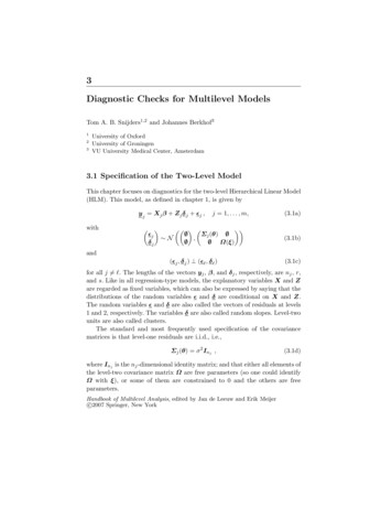
3 Diagnostic Checks for Multilevel Models149the assumption that the expected value of the residuals is indeed 0. Thereforethese heteroscedasticity checks should be performed only after having ascertained the linear dependence of the fixed part on the explanatory variables.To check linearity and homoscedasticity as a function of explanatory variables, if the plot of the residuals just shows a seemingly chaotic mass of scatter,it often is helpful to smooth the plots of residuals against explanatory variables, e.g., by moving averages or by spline smoothers. We find it particularlyhelpful to use smoothing splines [cf. 21], choosing the smoothing parameterso as to minimize the cross-validatory estimated prediction error.If there is evidence of inhomogeneity of level-one variances, the level-onemodel is in doubt and attempts to improve it are in order. The analysis of levelone residuals might suggest non-linear transformations of the explanatoryvariables, as discussed in the second half of this chapter, or a heteroscedasticlevel-one model. Another possibility is to apply a non-linear transformationto the dependent variable. Atkinson [2] has an illuminating discussion ofnon-linear transformations of the dependent variable in single-level regressionmodels. Hodges [28, p. 506] discusses Box-Cox transformations for multilevelmodels.As an example, consider the data set provided with the MLwiN software[19] in the worksheet tutorial.ws. This includes data for 4059 students in 65schools; we use the normalized exam score (normexam) (mean 0, variance 1)as the dependent variable and only the standardized reading test (standlrt)as an explanatory variable. The two mentioned uses of the OLS level-oneresiduals will be illustrated.Table 3.1. Parameter estimates for models fitted to normalized exam scores.Model 1Fixed partconstant termstandlrtstandlrt2standlrt3Random partLevel 2: ω11Level 1: σ 2Level 1: θ2devianceModel 2Model 30.0020.563(.040)(.012) 0.0170.6040.017 0.013(.041)(.021)(.009)(.005) 0.0170.6050.017 .095(.019)0.564(.013) 05)When the OLS within-cluster residuals are plotted against the explanatoryvariable standlrt, an unilluminating cloud of points is produced. Thereforeonly the smoothed residuals are plotted in Figure 3.1.

150Snijders and Berkhof0.20ǫ̂0.00 0.20 2.500.002.50standlrtFig. 3.1. Smoothing spline approximation for OLS within-cluster residuals (ǫ̂) underModel 1 against standardized reading test (standlrt).This figure shows a smooth curve suggestive of a cubic polynomial. Theshape of the curve suggests to include the square and cube of standlrt asextra explanatory variables. The resulting model estimates are presented asModel 2 in Table 3.1. Indeed the model improvement is significant (χ2 11.0,d.f. 2, p .005).As a check of the level-one homoscedasticity, the semi-standardized residuals (3.9) are calculated for Model 2. The smoothed squared semi-standardizedresiduals are plotted against standlrt in Figure 3.2.This figure suggests that the level-one variance decreases linearly with theexplanatory variable. A model with this specification (cf. section 3.2.1),Var(ǫij ) σ 2 θ2 standlrtij ,is presented as Model 3 in Table 3.1. The heteroscedasticity is a significantmodel improvement (χ2 4.8, d.f. 1, p .05).3.3.2 Homogeneity of Variance across ClustersThe OLS within-cluster residuals can also be used in a test of the assumptionthat the level-one variance is the same in all level-two units against the specificalternative hypothesis that the level-one variance varies across the level-twounits. Formally, this means that the null hypothesis (3.1d) is tested againstthe alternative

3 Diagnostic Checks for Multilevel Models1510.65ǫ̌20.550.45 2.500.002.50standlrtFig. 3.2. Smoothing spline approximation for the squared semi-standardized OLSwithin-cluster residuals (ǫ̌2 ) under Model 2 against the standardized reading test(standlrt).Σj (θ) σj2 Inj ,where the σj2 are unspecified and not identical.Indicating the rank of X̌j defined in section 3.3.1 by rj , the within-clusterresidual variance is1s2j ǫ̂′ ǫ̂ .n j rj j jIf model (3.1d) is correct, (nj rj )s2j /σ 2 has a chi-squared distribution with(nj rj ) degrees of freedom. The homogeneity test of Bartlett and Kendall [4]can be applied here (it is also proposed in Raudenbush and Bryk [45, p. 264]PPand Snijders and Bosker [51, p. 127]). Denotingnj n ,rj r andls pooled X1(nj rj ) log(s2j ),n r j(3.10)the test statistic is given byH X n j rj 2log(s2j ) ls pooled .2j(3.11)Under the null hypothesis this statistic has approximately a chi-squared distribution with m̃ 1 degrees of freedom, where m̃ is the number of clusters

152Snijders and Berkhofincluded in the summation (this could be less than m because some smallclusters might be skipped).This chi-squared approximation is valid if the degrees of freedom nj rjare large enough. If this approximation is in doubt, a Monte Carlo test can beused. This test is based on the property that, under the null hypothesis, (nj rj )s2j /σ 2 has an exact chi-squared distribution, and the unknown parameterσ 2 does not affect the distribution of H because its contribution in (3.11)cancels out. This implies that under the null hypothesis the distribution of Hdoes not depend on any unknown parameters, and a random sample from itsdistribution can be generated by randomly drawing random variables c2j fromchi-squared distributions with (nj rj ) d.f. and applying formulae (3.10) and(3.11) to s2j c2j /(nj rj ). By simulating a sufficiently large sample from thenull distribution of H, the p-value of an observed value can be approximatedto any desired precision.3.3.3 Level-Two ResidualsThere are two main ways for predicting4 the level-two residuals δ j : the OLSmethod (based on treating them as fixed effects δj ) and the empirical Bayes(EB) method. The empirical Bayes ‘estimate’ of δ j can be defined as itsconditional expected value given the observations y 1 , . . . , y m , plugging inthe parameter estimates for β, θ, and ξ. (In the name, ‘Bayes’ refers to theconditional expectation and ‘empirical’ to plugging in the estimates.)The advantage of the EB method is that it is more precise, but the disadvantage is its stronger dependence on the model assumptions. The twoapproaches were compared by Waternaux et al. [59] and Hilden-Minton [27].Their conclusion was that, provided the level-one model (i.e., the assumptionsabout the level-one predictors included in X and about the level-one residualsǫj ) is adequate, it is advisable to use the EB estimates.Basic properties of the multivariate normal distribution imply that the EBlevel-two residuals are given by (using parameter estimates β̂, θ̂, ξ̂)δ̂ j E δ j

The HLM is itself already a quite general model, a generalization of the General Linear Model, the latter often being used as a point of departure in modeling or conceptualizing effects of explanatory on dependent variables. Accordingly, checking and improving the specification of a multilevel model