Transcription
U.U.D.M. Project Report 2009:13Short rates and bond prices in one-factor modelsMuhammad Naveed NazirExamensarbete i matematik, 30 hpHandledare och examinator: Johan TyskJuni 2009Department of MathematicsUppsala University
ii
AcknowledgementAll prays to Almighty Allah who induced the man with intelligence, knowledge and wisdom.It is He who gave me ability, perseverance and determination to complete this thesis.Teachers are lighthouses spreading the light of knowledge and wisdom everywhere and guidingthe new generation so that they can cruise safely towards their destination. They areperforming the job, which Allah himself acknowledge as the noblest to all jobs; the job ofteaching. They will get its reward not only from Allah but also in the form of immense respectthat every student carries for them in the core of his heart.I offer my sincerest thanks and deepest gratitude to my research supervisor Prof. Johan Tyskfor his inspiring and valuable guidance, encouraging attitude and enlightening discussionsenabling me to pursue my work with dedication.I would like to say a big thanks to all the teachers who taught me during the entire program.They did not only teach me how to learn, they also taught me how to teach, and theirexcellence has always inspired me.I would like to take this opportunity to thank my colleagues, friends who were always there forevocative discussions, invaluable advice and support.Many thanks and my deepest gratitude to my parents who have kept me motivated through theextreme hard time and encourage me during the good times.iii
AbstractInterest rate modeling has gained special attention during the last few decades whichhas resulted in reliable models. These models are in common use for future evolution ofinterest rate; one way to accomplish this task is by describing the future evolution of the shortrate. The goal of the thesis is to provide a detail analysis of bond pricing using one factor shortrate model. The thesis explores and provides an insight into the practicality and the intervariability between different models.iv
Table of ContentsTable of Contents . 112Introduction . 2Basics Definition. 32.12.22.32.4Bond Types . 4Bond price . 6Bond Yield . 62.6Relation between Yield and Bond Price . 6Bond Convexity and Duration. 9One Factor Short Rate Models . 103.1Short Rate Model . 103.2Vasicek Model . 103.3The Hull White Model (Extended Vasicek Model) . 163.43.53.63.74Bond Characteristics . 32.52.73Bond . 3Cox Ingersoll Ross Model . 19The Hull White Model (Extended CIR Model) . 23Dothan Model . 24Black-Derman-Toy Model. 26Model’s Evaluation . 284.14.24.34.4Vasicek Model . 28Extended Vasicek Model . 28Cox Ingersoll Ross Model . 29Extended Cox Ingersoll Ross Model . 294.5Black Derman Toy Model . 294.6Short Rate Model Versus Other Models. 30Conclusion: . 31References . 321
1 IntroductionThis thesis defines and analyzes a simple one-factor model of the term structure ofinterest rates. The issue of pricing interest rate derivatives has been addressed by thefinancial literature in a number of different ways. One of the oldest approaches is basedon modeling the evaluation of the instantaneous short interest rate. This is still quitepopular for pricing interest rate derivatives and for risk management purposes, andrepresents the most commonly used type of dynamical stochastic model for interest rates.Therefore, one of the aims of this study is to give information about these models andallow readers to compare them.In this thesis, we are discussing on-factor short rate models, Vasicek model (1977), Hull-White (extended Vasicek model) (1993), Cox Ingersoll Ross model (1985), Hull-White(extended CIR model) (1993), Dothan model (1978), Black-Derman-Toy model (1980).The thesis is organized as follows: Chapter 2 provides with the basic introduction tobonds. The Chapter to follow will discuss different short rate models for bond pricing.Finally, Chapter 4 summarises the results and discussions with concluding remarks.2
2 Basics Definition2.1 BondA bond is a debt instrument which is issued for a period of more than one year for thepurpose of capital rising by borrowing. A bond is a promise to repay the principal withinterest (coupons) on a specific date (maturity). Some bonds do not pay interest but allbonds require a repayment principal.2.2 Bond CharacteristicsA bond depends on the following characteristics, IssuersBonds are issued by public authorities, credit institutions, companies andsupranational institutions in the primary markets. The most common process ofissuing bonds is through underwriting. In underwriting, one or more security firmsor banks, forming a syndicate, buy an entire issue of bonds from an issuer and resell them to investors.There is little difference between bonds issued by companies and those issued bythe national government. A federal government bonds have a low risk by default,where as corporate bonds are considered higher risk. International bonds arecomplicated by different currencies. These types of bonds are issued in foreignmarket to the issuer’s home market and the currency type is the currency of theforeign market. Examples of some international bonds are Euro bonds, Foreignbonds, Global bonds etc. PriorityDetermined by the probability of when the issuer will pay back the money. Thepriority shows your place in the queue of the company for payments. If you haveunsubordinated (senior) security then you will be the first in the queue to receive3
payment from bankruptcy of its assets. But if you have subordinated (junior) debtsecurity then you will receive payment after the senior (unsubordinated) securityholders have received their shares. Coupon Rate (Interest Rate)Interest payment received by the bondholder is called “coupon”. Most bond issuercompanies pay interest every sixth month, but it is also possible to pay monthly,quarterly or annually. The coupon is expressed as a percentage of its value. If thebond coupon rate is fixed (or stays fixed) and market rate rises then bond price arereduced or if market rate falls then bond price will rise. RedemptionThe return of an investor's principal in a security, such as a stock, bond, or mutualfund. Or we can say as, both investor and issuers are exposed to interest rate risksbecause they agree either to receive or pay a set coupon rate over a specific period oftime.2.3 Bond Types Callable (Redeemable) bond gives rights to bond issuer but not obligation toredeem his issue of bonds before its maturity. Issuers have to pay bond holderspremium. There are two types of this bond.o American Callable bonds can be called by the issuer any time after the callprotection.o European Callable bonds can be called by the issuer only on pre-specified dates. Convertible bonds give rights to bondholder but not obligation to convert theirbonds into different securities, like shares. This only applies on corporate bonds. Puttable bonds give rights to bondholder but not obligation to sell their bonds backto the issuer at a predefined date and price. Investors can ask for the repayment ofthe bond.4
Asset-Backed Securities are bonds or currency notes secured by assets of thecompany. “It is defined as yield and redemption are guaranteed by assets of theissuer, exclusively earmarked for the satisfaction of the rights incorporated in thefinancial instruments themselves”, [Ref. 10]. Corporate bonds are debt securities issued by the corporation. Like all bonds, theirvalues rise when market interest rate falls and fall when market interest rate rises.They involve risk of principal. Euro bonds are medium or long term interest bearing bonds created in internationalcapital markets. It is dominated in a currency other than the place where it is issued.It is also called global bond. Junk Bonds (high yield bonds) are issued from risky companies. So they offerhigher interest rates to compensate the risk. Municipal bonds are issued by various cities having some low interest rates andthese bonds are tax free. Zero-Coupon bond (also called discount bond) is a bond that is redeemed at fullface value at the maturity date ‘T’. This is special type bond that does not pay tax.The price at time t of a bond with maturity date ‘T’ is denoted by p (t, T). Weassume that Market (frictionless) for T-bonds for every T 0 . p ( t , t ) 1 t. For fixed t, the bond price p ( t , T ) is different with respect to ‘T’ (time ofmaturity). Calculated Zero coupon bond price M(1 i ) n5
2.4 Bond priceA good sum is paid to buy a bond. Bond prices have an inverse relationship withinterest rates. When interest rates rise, bond prices fall and when interest rates fall,bond prices rise. Here is the formula for calculating a bond’s price, i.e. basic PresentValue (PV) formula:Price CCCM, . 2n(1 i )(1 i )(1 i )(1 i ) nC Coupon, n no. of paymenti interest rate, M value at maturity2.5 Bond YieldThe return received when bond is purchased and held to maturity. The yield iscalculated by dividing the interest rate by the purchase price of the bond.2.6 Relation between Yield and Bond PriceYield is the return on an investment, expressed as annual percentage. For example 3%yield means that the averages 3% of investment is returned each year. There are severalmethods to calculate yield. Current YieldThe simplest way to calculate the current yield isCurrent Yield Annual Interest ( )*100 ,pricewhile current yield is easy to calculate, however it is not as accurate a measure asyield to maturity. So the modified current yield formula that takes into discount/ premium account for bond is AnnualCoupon (100 Market Pr ice) Adjusted Current Yield *100 , Marketprice Year.to.Maturity now the current yield for zero coupon bonds, which has only one couponpayment, is6
1 Future Value n Yield 1, Purchase Pr ice Where n years left until maturity. Yield to MaturityThe current yields return the annual coupon payment, but this percentage doesnot take into account the time value of money. Yield to maturity (YTM) is theinterest rate which is the present value of all cash flows. And cash flows areequal to the bond’s price. YTM require a complex calculation. It considers thefollowing factors. Coupon rate: Higher bond’s coupon rates have higher yield. Price: Higher bond’s price, the lower yield. Remaining Year until maturity: By reinvesting the interest payment, canearn more bonds.The difference between the face value and the price is that if you keep a bond tomaturity then you get the face value of bond. You might get less or more theprice you paid. Yield to maturity can be calculated as, 1 1- n (1 i ) 1 Bond Price cashflow *, Maturity*i(1 i) n here, i Interest rate. Calculating yield for callable and puttable bondThe yield for callable bond is also called yield-to-call and the yield for puttablebond is also called yield-to-put. Yield-to-Call and Yield-to-put is a Yield toMaturity assuming that the bond will redeem at the Call or Put date. It can becalculated as7
P 100R iMY Y i 1 1 1 100 100 M . Yield to WorstThe lowest yield calculated is known as yield to worst. We can assume as if theissuer does not default. If market yields are higher than the coupon, the yield toworst would assume no prepayment. If market yields are below the coupon, theyield to worst would be assuming prepayment. We can say as, yield to worst thatmarket yields are unchanged. Yield Curve and Maturity DateA yield curve is the relationship between interest rates and time, determined byplotting the yields of all default-free coupon bonds against their maturities. Theyield curve typically slopes upwards since longer maturities normally have higheryields, although it can be flat or even inverted. Normal Yield CurveA normal yield curve is a graph, illustratingthe structure of interest rates over a periodof time, which indicates that rates rise asmaturities lengthen, i.e., short-term rates arelower than long-term rates. It is also knownas “positive and upward-sloping” yield. Flat Yield CurveA yield curve in which there is little differencebetween short term and long term rates forbonds of the same credit quality. Or a yieldcurve showing same yield for short maturity andlong maturity bonds called Flat Yield Curve.8
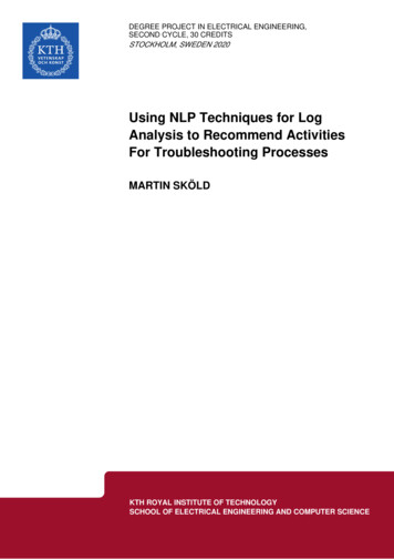
Inverted Yield CurveA rare situation, where long term interestrates have lower yields and short terminterest rates have a negative yield curve(interest rates decrease as maturitieslengthen).A negative yield curve is a graph, depicting the structure of interest rates overtime, which indicates that as maturities lengthen interest rates fall, short-termrates exceed the long-term rates. Spot Rate curveIt is the graphical depiction of the relationship between the spot rates andmaturity.2.7 Bond Convexity and DurationAs bond yields go higher, the price goes lower. This relationship between price andyield has a convex structure in nature. The term used to describe this relationship isalso known as convexity.Bond convexity is the sensitivity of Bond duration to changes in interest rates. Bondduration is the sensitivity of Bond prices to change in interest rates. In calculus terms,duration is the first derivative of the price/yield equation and convexity is the secondderivative.9
3 One Factor Short Rate Models3.1 Short Rate ModelThe short rate describes the future evolution of the interest rate by describing the futureevolution of the short rate.The short rate ( rt ) is the interest rate at which an entity can borrow money for a shortperiod of time from time t. The current short rate does not specify the entire yieldcurve. However no-arbitrage arguments show that, under some fairly relaxed technicalconditions, if rt as stochastic process under a risk-neutral measure (Q) then the price attime (t) of a zero-coupon bond maturing at time T is given by()T P (t,T ) Ε exp rs ds Ft ,t (3.1.1)where F is the natural filtration for the process, thus specifying a model for the shortrate specifies future bond prices. This means that instantaneous forward rates are alsospecified by the usual formula.f(t,T ) ln ( P ( t , T ) ) . T(3.1.2)Here we consider models for the short rate with only one source of randomness, socalled one-factor models.3.2 Vasicek ModelThe Vasicek model was introduced by Oldrich Vasicek in 1977 [8]. This model can beused for interest rate derivative valuation and also adapted for credit market, although ituses the wrong principle for credit market and implying negative probabilities [11].Vasicek Model is an Ornstein-Uhlenbeck stochastic process.10
This model specifies that the instantaneous interest rate follows the stochasticdifferential equation.drt a ( b rt) dt σ dWt . Here Wt is a Wiener process, modelling the random market risk factor. σ (Standard deviation parameter), determines the volatility of the interest rate. ) , is the drift factor that describes the expected change in the interest rateat that particular time. b: “Long term mean value”. The long run equilibrium value towards which thea ( b rtinterest rate goes back. a: “Speed of reversion”. It gives the adjustment of speed and has to be positive inorder to maintain stability around for the long-term value. For example, when rt is below b, then the drift term a ( b rt ) becomes positivefor positive a, generating a tendency for the interest rate to move upwards (towardequilibrium). Note that X { X t } with X t rt b is an Ornstein-Uhlenbeck (O-U) processsatisfying the SDEdX t aX t dt σ dWt .Hence X is a Gaussian process, which implies Q ( rt 0) 0 for every t [ 0, T ]an unreasonable behaviour in practice. Pricing of bond option would be easybecause nice properties of the O-U process.Vasicek model was the first economics model to capture the value of mean reversion.Mean reversion is an important characteristic of the interest rate that is responsible toset it apart from other financial prices. Hence interest rates neither rise nor decrease11
indefinitely unlike stock prices. It moves within a limited range, showing a tendency torevert to a long run value. It gives an explicit formula for the (zero coupon) yield curveand gives explicit formulae for derivatives such as bond option. It can be used to createan interest rate tree. Calculating Bond Price Implied by the Short RateThe Vasicek Model assumes that the short rate rt , under risk-neutral measure isgiven bydrt a ( b rt) dt σ dWt .(3.2.1)Here a, b & σ are positive constant. We obtain after integratingttrt e at r0 abe au du σ e au dWu ,00 t e at r0 b ( e at 1) σ e au dWu , 0 µt σ 0 e a ( u t ) dWu ,twhere µt is a deterministic function and E [ rt ] µt . The expected value E [ rt ]can be determined without explicitly solving the SDE. Let’s take integral forequation (3.2.1).rt r0 ( a ( b ru ) du σ dWu ) ,t0Thenµt : E [ rt ] r0 a ( b E [ ru ]) d u,t0(3.2.2)d µt a ( b µt ) .dtThis is a linear ordinary differential equation (ODE). Now we use theintegrating factor e at . That is12
µt E [ rt ] e at r0 b ( e at 1) ,Further we can define it,(t E σ e at dWu0 t σ 2 e at E e 2 au du , 0 σ t2 :Var[ rt ] 1 e 2 at σ2 2a(3.2.3)) ,2 . Since normal random variables can become negative with positive probability,this is a weakness of Vasicek model. Now using the risk-neutral valuationframework, the price of a zero-coupon bond with maturity T at time t is(Now consider that)TE exp ru du Ft ,t B (t,T )X ( u ) ru b .(3.2.4)X ( u ) is the solution of the Ornstein-Uhlenbeck equation, sodX ( t ) aX ( t ) σ dWt ,with X ( 0 ) r0 b . Applying Itô’s lemma formula, then the X (u) is given by()X ( u ) e au X (0) σ e as dWs . u0(3.2.5)Here we can see that X (u) is a Gaussian process with continuous sample paths.Thus t0X (u )duis also Gaussian process. E ( X ( u ) ) X ( 0 ) e au , thentX ( 0)E X ( u ) du (1 e at ) , 0 a(3.2.6)13
now the variance istttVar X (u )du Cov X (u )du , X ( s )ds ,0 0 0 ttt t E X (u )du E X (u )du X ( s )ds E X ( s )ds , 0 0 0 0after solving it, we get,σ2 2a 3( 2at 3 4e at e 2 at ) .(3.2.7)From equation (3.2.4), we getttE ru du E ( X ( u ) b ) du . 0 0 (3.2.8)Now combining equation (3.2.8) with (3.2.6), we gettr b tE ru du 1 e a (T t ) b ( T t ) , 0 a(And)(3.2.9)TTVar ru du Var X (u )du , t t σ22a3( 2a (T t ) 3 4eNow the zero coupon bond is, a (T t )) e 2 a(T t ) .(3.2.10))(E exp ( r ( r ) du ) . TB ( t , T , rt ) E exp ru du rt , t TtutHere ru is a function of rt , so combining equation (3.2.9) and (3.2.10), andgetting the bond price14
TT1 B ( t , T , rt ) exp E ru ( rt ) du Var ru ( rt ) du , tt 2 2 rt b σ a (T t ) a T t 2 a T t1 e exp b (T t ) 3 2a (T t ) 3 4e ( ) e ( ) ,a 4a ()() 1 e a (T t ) 1 e a (T t ) σ 2 1 e a (T t ) σ 2 (T t ) 2 rt b 2 (T t ) aaa 2a 2a exp , a (T t ) 2 a (T t )2 σ12ee 2 4a a σ2σ2σ22 exp A ( t , T ) rt b At( , T ) b (T t ) 2 A ( t , T ) 2 (T t ) A ( t , T ) ,2a2a4a we get exp ( A ( t , T ) rt D ( t , T ) ) ,whereA (t,T ) 1 e a (T t )a(3.2.11)andσ 2 A (t,T ) σ2 D ( t , T ) b 2 A ( t , T ) (T t ) .24aa 2So by the result of equation (3.2.7), rt represent the Itô integral. The equation(3.2.11) is called an exponential affine bond price. The simple Gaussianstructure of rt (short rate process) leads to a closed form solution of the bondprice.Conclusions: The model is arbitrage free, in that sense, no bond or option priceproduced by the model will allow or permit arbitrage.15
As a one-factor model, it does not capture the mode complex termstructure shifts that occur. The main disadvantage is, (under the theory) the value of interest ratecan be negative.The Hull-White Model is the further extension over Vasicek Model.3.3 The Hull White Model (Extended Vasicek Model)In Vasicek model, we found the poor fitting of the initial term structure of interest rate.So, for the need of exact fit, The Hull-White model introduced by “Johan C.Hull andAlan White” in 1990 [7]. It is a model of future interest rate. It belongs to the class ofno-arbitrage models that are able to fit today’s term structure of interest rate. The HullWhite model is varying the time parameter in Vasicek model. It allows the deviation ofanalytical formulae that is strength of its normal distribution. But weakness is that, italso allows the negative interest rate with positive probability.This model is short rate model. So, the stochastic differential equation for the extendedVasicek Model is written asdrt ( a ( t ) b ( t ) rt ) dt σ ( t ) dWt .(3.3.1)Here, Wt is a Brownian motion in the martingale measure. We will consider thismodel when a a ( t ) but “b” and “ σ ” are constants.tLet K t au du and applying Itô’s lemma integration by parts to e Kt rt ,0()d e Kt rte Kt K t' rt dt e Kt drt ,(3.3.2)therefore16
()d e Kt rt e Kt bt rt dt e Kt ( at bt rt ) dt σ t dWt , e Kt bt rt dt e Kt at dt e Kt bt rt dt e Kt σ t dWt , e Kt at dt e Kt σ t dWt , e Kt ( at dt σ t dWt ) ,and integrative,te K rt r0 t0te Ku au du e Ku σ u dWu ,0(tt00)rt e Kt r0 e Ku au du e Ku σ u dWu ,rt e Kt r0 e(t Kt Ku )0au du e(t Kt Ku )σ u dWu .0(3.3.3)To generalize the result for any u t , so we havert e ( t K Ku )tr0 e ( Kt Ku )0tau du e ( Kt Ku )0σ u dWu ,(3.3.4)usually b ( t ) and σ ( t ) are supposed to be constant so the equation (3.3.4) will bert e bt r0 e b( t u ) au du e b( t u )σ u dWu ,(3.3.5)rt e b( t s ) rs e b( t u ) au du e b( t u )σ u dWu ,(3.3.6)tt00ttssFor bond priceIn the term structure, a discount bond with S-time, T-maturity value hasdistribution aswhereB ( S,T ) P ( S , T ) A ( S , T ) exp ( B ( S , T ) r ( S ) ) ,1 exp ( b (T S ) )b(3.3.7),17
2 log ( P ( 0, S ) ) σ 2 ( exp ( bT ) exp ( aS ) ) ( exp ( 2aS ) 1) P ( 0, T ) , A ( S , T ) exp B ( S , T ) P ( 0, S )dS4a 3 V ( t ) P ( t , S ) Φ ( d1 ) KP ( t , T ) Φ ( d 2 ) .To fit this model to the initial term structure of interest rate, we have to calculatethe zero coupon bond prices. We have shown that the price of a zero coupon bondat present with T-maturity is P ( 0, T ) E Q e 0 Tlet consider y ( t ) t0rs ds , (3.3.8)rs ds , so above equation will be(P ( 0, T ) E Q e y (T )).(3.3.9)By using equation(3.3.5), y ( t ) can be calculated, bty (t ) e r0 ds andtt00 s0e b( s u )au duds t0 s0e b( s u )σ u dWu ds ,r0 ( e bt 1) t t b( s u )t t b s uy (t ) eau duds e ( )σ u dWu ds ,0 u0 ubr0 ( e bt 1) bs t buty (t ) e e au ( t u ) du e bs ebuσ ( t u ) dWu .00b(3.3.10)From the short rate dynamics of Hull-White, it is easily seen that the interest ratesare normal. So y ( t ) t0rs ds is a sum of normal distributed random variables.Therefore, it is also normal distribution. So, y ( t ) has mean withand variancer0 ( e bt 1)tm (t ) e bs ebu au ( t u ) du ,0b18
t2te 2bt1 v ( t ) e 2bsσ 2 2 3 3 .4b4b 2b 2bFrom the expression of the Laplace transform of Gaussian, the equation (3.3.9) canbe written as1 exp E Q ( y (T ) ) Va r( y (T ) ) , 2 we also know that exp m ( T ) 1v (T2(3.3.11)) , after substituting values in the equation, then we get r0 ( e bt 1) T e bs ebu au (T u ) du 0b , exp 22 bT 1 T1 Te e 2 bsσ 2 233 22244bbbb (3.3.12)taking the logarithms and differentiating twice time with respect to ‘T’. Using theequality of the instantaneous forward rate, f ( 0, T ) get ‘a’ asa (T ) log P ( 0, T ), we can T f ( 0, T )σ2 bf ( 0, T ) 1 e 2bT ) .( T2b(3.3.13)3.4 Cox Ingersoll Ross ModelThe Cox Ingersoll Ross model was introduced in 1985 by ‘John C. Cox, Jonathan E.Ingersoll and Stephen A. Ross’ as an extension of the Vasicek Model [6].The CIR bond pricing model assumes that the risk natural process for the Shortinterest rate is given bydr a ( b r ) dt σ rdWt .19
a ( b r ) is the same as in the Vasicek Model. The standard deviationfactor σrt , avoid the possibility of negative or null rates if the condition2ab σ 2 is met.The CIR model specifies that the interest rates follow the stochastic differentialequation,drt a ( b rt ) dt σrt dWt ,(3.4.1)ttuu(3.4.2)taking integralrt r a ( b rs ) ds σ uApplying Itô’s lemma f( xt ) xt2rs dWs ,and xt rt , so equation will be1rs .dWs 2σ 2 rs .ds ,2 uttru2 2rs abds ars ds σ rs .dWs σ 2 rs .ds , uurt 2 ru2 2rs a ( b rs ) ds σuttttuu ru2 2rs abds 2ars2 ds 2σ . 3 rs .dWs σ 2 rs .ds , ru2 tuand( 2r ab 2ar2ss σ 2 rs ) ds 2σ . 3 rs .dWs ,turt ru2 ( 2ab σ 2 ) rs ds 2a rs2 ds 2σ If µ 0 thentttuuurt r0 a ( b rs )ds σ Thus, the unconditional mean istt00(rs .dWs .3rs .dWs ,(3.4.3)(3.4.4))E Q ( rt ) r0 a bt E Q ( rs ) ds ,t020
()solving the equation Φ ( t ) r0 a bt Φ ( s ) ds , which can be transformedt0into the ODE (ordinary differential equation) Φ ( t ) aΦ ( t ) ab .'So, the unconditional mean isE Q ( rt ) b ( r0 b ) e at ,can also write as,{(}(3.4.5))E Q rt Furu e a( t u ) b 1 e a( t u ) .Similarly, we can write equation (3.4.3) asE Q ( rt 2 ) r02 ( 2ab σ 2 ) E Q ( rs2 ) ds 2a E Q ( rs2 ) ds ,tt00(3.4.6)substituting the value of E Q ( rt ) into (3.4.6) and applying second derivative, then wecan get varianceVar ( rt ) or{} Var rt Fuσ2a(1 e ) r e( (ru σ 2 e bt0 a ( t u )a e bt b 1 e bt ) ,(2 2 a ( t u )(3.4.7)) ) bσ (1 e2 a ( t u )2a)2.In [6], they aimed to have relationship between term structure of interest rates andyields on risk free securities that differ only in their time to maturity. The explanationof the term structure gives extra information to predict the effect on the yield curve ifwe change the underlying variables.The instantaneous short rate dynamics corresponds to a continuous time first-orderautoregressive process where the randomly moving interest rate is elastically pulledtoward a central location or long term value, b, which leads to mean reversion property.If σ 2 2ab then rt can be zero.If σ 2 2ab then the upward drift is sufficiently large to make the originalinaccessible.21
So from (3.4.7) equation we get that there is no explicit form for the solution to theCIR model. It is known that the model has unique positive solution. If the interest ratereaches zero then it can subsequently become positive.More generally, when the rate is low (close to zero), then the standard deviation alsobecomes close to zero.For calculating the increment of bond price in the volatility of CIR model, we use theformulation under the risk-neutral measure ‘Q’ is drt a ( b rt ) dt σrt dWt .We assuming here, a pure discount bond p
Interest payment received by the bondholder is called "coupon". Most bond issuer companies pay interest every sixth month, but it is also possible to pay monthly, quarterly or annually. oupon is expressed as The c a percentage of its value. If the bond coupon rate is fixed (or staysfixed) and market rate rise then bs ond price are